Published by Canadian Center of Science and Education
The Identification of Gas-liquid Co-current Two Phase Flow Pattern
in a Horizontal Pipe Using the Power Spectral Density and the
Artificial Neural Network (ANN)
Budi Santoso1,4, Indarto2, Deendarlianto2 & Thomas S. W.3 1
Graduate Program of Mechanical and Industrial Engineering, Faculty of Engineering, GadjahMada University, Indonesia
2
Department of Mechanical and Industrial Engineering, Faculty of Engineering, GadjahMada University, Indonesia
3
Departmen of Electrical Engineering and Information Technology, Faculty of Engineering, GadjahMada University, Indonesia
4
Department of Mechanical Engineering, Faculty of Engineering, SebelasMaret University, Indonesia
Correspondence: Budi Santoso, Department of Mechanical Engineering, Faculty of Engineering, SebelasMaret University, Jl. Sutarmi 36A Surakarta 57126, Indonesia. E-mail: [email protected]; [email protected]
Received: July 23, 2012 Accepted: August 18, 2012 Online Published: August 29, 2012 doi:10.5539/mas.v6n9p56 URL: http://dx.doi.org/10.5539/mas.v6n9p56
Abstract
This paper presents a new method of the flow pattern identification on the basis of the analysis of Power Spectral Density (PSD) from the pressure difference data of horizontal flow. Seven parameters of PSD curve such as mean (K1), variance (K2), mean at 1-3 Hz (K3), mean at 3-8 Hz (K4), mean at 8-13 Hz (K5), mean at 13-25 Hz (K6) and mean at 25-30 Hz (K7) were used as training vector input of Artificial Neural Networks (ANN) in order to identify the flow patterns. From the obtained experimental of 123 operating conditions consisting of stratified flow, plug and slug, ANN was trained by using 100 data operation and 23 tested data. The results showed that the new method has a capability to identify the flow patterns of gas-liquid two phase flow with a high accuracy.
Keywords: flow pattern identification, power spectral density (PSD), artificial neural network (ANN), two phase flow
1. Introduction
The knowledge of two phase flow is of important in engineering process, such as oil industry, chemical process, power generation, and phase change heat exchanger apparatus. The common characteristics of parameter related to the flow pattern are the pressure gradient and the void fraction. The main issue in two phase flow researches is the relationship between the pressure fluctuation and flow pattern. In general, the pressure fluctuations resulted from the liquid-gas flow and their statistical characteristics are very interest for the objective characterization of the flow patterns because the required sensors are robust, inexpensive and relatively well established, and therefore more likely to be implemented in the industrial systems (Drahos et al., 1991).
Artificial Neural Network (ANN) provides an alternative method for either modeling phenomena which are too difficult to model from fundamental principles, or reduce the computational time for predicting expected behavior. Artificial neural network is based on the important rules for classifying the flow pattern. Neural network stimulate human mind and demonstrate high intelligence and it can be trained to study the correct output and classify training exercises. Here, neural network needs knowledge input for training. After the training, the neural network can classify the similar flow pattern with a high accuracy.
Cai et al. (1994) applied the Kohonen self-organizing neural network in order to identify the flow pattern in a horizontal air-water flow. In their work, the neural network was trained with stochastic features derived from the turbulent absolute pressure signals obtained across a range of the flow regimes. The feature map succeeded in classifying samples into distinctive flow regime classes consistent with the visual flow regime observation. Next, Wu et al. (2001) recorded the pressure difference signal in pipe flow and used the fractal analysis to analyze them for identification of flow pattern. By using the ANN, the good result was obtained but it is only considered stratified, intermittent and annular flows. For this reason, Jia et al. (2005) proposed a new flow pattern identification method based on PDF and neural network at the horizontal flow in pipe.
Xie et al. (2004) examined the feasibility of the implementation of the artificial neural network (ANN) technique for the classification of flow regimes in three phase gas/liquid/pulp fiber systems by using the pressure signals as input. For this purpose, the flow behavior by using the power spectral density function is needed to implement the parameterization of the information contained in the spectral patterns.
Table1. The experiment conditions using pressure sensor Authors System Diameter/
Orientation Measurement technique Method and finding Franca et al.
(1991)
Water-air (wavy, plug, slug and annular)
D=19 mm; horizontal
Pressure drop, XDP=8D, N=5 000
Using fractal techniques for flow pattern identification and classification. Cai et al.
(1994)
Water-air (stratified, slug, intermittent transition, and bubble)
D= 50 mm; horizontal
Two absolute pressure, XDP=1D, SR=40Hz, N=40 000
Kohonen self-organizing neural network to identify flow regimes.
Drahos et al. (1996)
Water-air (plug and slug)
D=50 mm; horizontal
wall pressure
fluctuations, XDP=8D, SR=500Hz, N=60 000
Chaotic time series analysis to obtain a new insight into the dynamics of the intermittent flow pattern. Wu et al.
(2001)
Oil-gas-water, (stratified, intermittent and annular)
D= 40 mm; horizontal
Differential pressure, XDP=5D,
The fractal analysis to analyze the signal for identification of flow pattern.
Jia et al. (2005)
Water-air (stratified, churn, slug, annular)
D= 32 mm; horizontal
Differential pressure, XDP=10D, SR=200Hz, N=6 000
Flow pattern identification method based on PDF and neural network.
Matsui et al. (2007)
Water and nitrogen gas (small bubble train, plug and slug)
D= 7 mm; horizontal
Differential pressure, XDP=1D, XDP=7D SR=100Hz, N=2 000
The flow pattern, the void fraction and the velocity of gas phase were measured by PDF and cross correlation. Hao et al.
(2007)
Water-air, (wavy, bubble, plug and slug)
D=15 mm, 25 mm, 40 mm; horizontal
Differential pressure, XDP=250mm,
SR=200Hz, N=30 000
The application of the Hilbert–Huang Transform (HHT) to identify flow regimes.
Xie et al. (2004)
Gas-liquid-pulp fiber (churn, slug)
D= 50.8mm, vertical
Local pressure
fluctuations, SR=200Hz, N=2 000
The summ
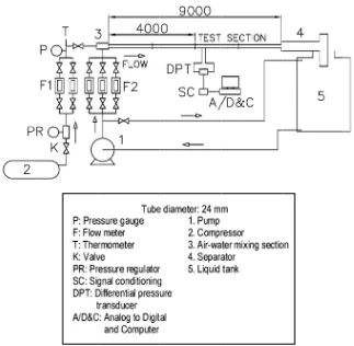
Figure 1 sh compresso are as follo m/s.
3. Results
3.1 Flow P
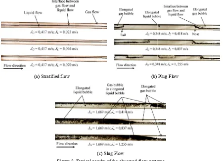
Figure 2 sh and (c) cor
mary of experim e tap (mm), SR entification, di ave contributed of researchers propagation ne was designed, stics of the po e flow regimes
ments Appara
hows a schema or and water ly by flow me d into the atmo inner diameter
n in the Figure r with 5D dista r were sent thr g time of exper ows: the range
and Discussi
Patterns
hows the typic rrespond to int
ment condition R is sampling r istance of pre d to our unde in flow patter eural network
trained and te ower spectrum s with good acc
atus and Proc
atic diagram o from pump eters. The air-w osphere and wa r and of 9 m to
Figure 1. Sc
e 1, the press ance of pressur rough amplifie rimental run w e of superficia
ons
cal results of th terfacial behav
ns from the pre rate and N is s essure tap, sam erstanding of f rn identification
was used to i ested for the cl for one of the curacy.
cedure
of the experime into an air-w water mixture
ater is measure otal length is m
chematic diagr
sure fluctuatio re tap. The tran er into a comp was 50 s. The w al air and wate
he flow pattern vior of the strat
evious research size of data. It mpling rate, si flow patterns n. In this pape identify flow p lassification of e normalized d
ental apparatus water mixing
flows through ed more accur made of transpa
ram of the exp
n was detecte nsducer has ± puter via A/D working fluids er velocities; J
ns obtained fro tified, plug and
her is shown i gave the infor ize of data an of two-phase er, the different
pattern of two f the flow regi differential pre
s used in the p section after h the tube into
rately by weigh arent acrylic re
perimental app
ed by Validyn 0.25% full sca converter. Sam were air and w G=0.085-3.204
om the present d slug flows, r
in Table 1, wh rmation about t nd flow pattern flows and los tial pressure, t
phase flow at imes using as essure signals
present study. A their flow ra an air-water s hing if necessa esin to observe
aratus
ne DP15-32 di ale accuracy. O mpling rate w water. The exp 4 m/s, and tho
experiment. T respectively. In
here XDP is dist the method of n identified. T sing the subje the analysis of t a horizontal
input some de and was show
Air supplied fr ates are meas separator, wher ary. A smooth e the flow patte
ifferential pre Output signals was 400 Hz an periment condi
se JL= 0.016-1
The Figures, (a n the stratified
the gas ph interfacial patterns. T of fluid. A of the tube same velo small diff magnitude the upper w at the high transported
hase travels alo waves. As sh The stratified fl As shown in th
e in a continuo ocity with the
ference betwee e of the waves
wall of the tub her velocity o d by the liquid rn is highly un en pressure pu
(a) Str
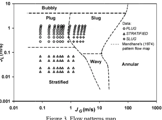
he obtained flo 4) as shown in ent with those
ong the upper h hown in Figure flow pattern oc he Figure 2(b) ous liquid flow
liquid, and th en the velocit increases. Th be to form som of the gas (Fig d phase, in slug ndesirable in p
lses and severe
ratified flow
Figure 2.
w pattern data n Figure 3. Clo
of Mandhane
half of the tub e 2(a), this flo ccurs at relative the plug flow w. Next, it is n he gas-liquid in
ties of the ph his condition is me liquid pack
gure 2(c)). Un g flow the liqu practical applic
e pressure osci
(c) . Typical resul
a is compared w ose observatio
et al. (1974).
e while the liq ow has the sim
ely low gas an is characteriz noticed that in nterface below hases at the in s called slug f kets, also liquid
nlike plug flow uid slugs are c cations. The fa illations that c
) Slug Flow lts of the obser
with the horizo on of this figur
quid flows alon mplest configu nd liquid mass ed by elongate n the plug flow w the bubbles nterface. With flow. Ultimatel d slugs. These w, in which th carried by the f aster moving li an cause dama
(b)
rved flow patte
ontal flow patt re reveal that th
ng the bottom uration of all t flow rates and ed bubbles flo w; elongated bu
is relatively s h the increase ly, the waves liquid slugs a he elongated b faster moving iquid slugs are age to downstr
Plug Flow
erns
tern map prop he obtained flo
with no signif the horizontal d density differ wing along th ubbles move a stable, indicati e gas velocity build up and r are then transp
bubbles of ga gas flow. The e usually assoc ream equipmen
posed by Mand ow pattern dat
Figure 4 sh
pressure d points and
3.2 Typica
In this pap the differe
hows the struc m of flow patte
data processin part of the syst
normalized pre
P is differenti different signal d a Hanning W
al Flow pattern
per, three typic ent of the flow rns are shown tified Flow es signal and
with a small f between water one peak and sp
cture of the int ern identificat ng unit. Differ tem, while dat
Figure 4. S
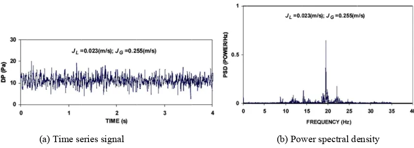
essure fluctuat
ial pressure ( l (Pa). The po Window of the s
n and Power Sp
cal flow patter w patterns. Ex
in Figure 5 to
PSD of strati fluctuation. Th
flow and air f preads over wi
Figure 3. F
telligent identi tion is compos rential pressur ta processing u
Structure of the
tions in the tim *
rns ware ident amples of tim
Figure 7.
fied flow is s his flow pattern
flow is clear (n ide frequency
Flow patterns
ification system sed of differen re measuring unit constitutes
e intelligent id
me series is defi (
) D
DP
DP
average differ m was estimate
ty
tified. The cha me series press
shown at Figu n occurs at low no bubble). Fro range from 8 t
map
m used in pres ntial pressure unit and data s the software p
dentification sy
fined below: 2 sure different a
ure 5, in which w superficial v
om Figure 5(b to 27 Hz.
sent study. As measuring un a acquisition part of the syst
ystem
re (Pa) and D
egments with
f their PSD we and power spe
h it shows a l velocities of wa b), it is reveale
shown in Figu nit, data acquis unit constitute tem.
DP* is norma a length of 16
ere used to ide ectra for the m
low mean pre ater and air an ed that the strat
Figure 5
3.2.2 Plug Figure 6 sh difference due to the divided int
Figure
3.2.3 Slug Figure 7 sh when com peaks valu range pres of peak va
(a) Time se . Typical of th
Flow hows the time
of plug flow h e air bubble h
to two parts. T
(a) e 6. Typical of
Flow hows the time mpared with the ue that it is ca sent the bubble alue decreases
eries signal he time variatio
variation of p has a bigger fl has a compres There are in the
) Time series s f the time varia
e series signal e stratified flow aused by the h es flow with ze
(see Figure 7(b
on of pressure
JG=
pressure gradie luctuation than sible effect th e range of 0-11
signal
ation of pressur JG=
and the PSD s w and plug flow high water vel ero value. PSD
b)).
gradient and th =0.255 m/s
ent and the PSD n that of stratif hat cause large
1 Hz and 11-27
re gradient and =0.438 m/s
slug flow. Slug w, as shown in locity pushing D of slug flow h
(b) Pow he PSD in stra
D of plug flow fied flow as sh e fluctuations. 7 Hz (see Figu
(b) Powe d the PSD in p
g flow time se n Figure 7(a). g the elongated
has the frequen
wer spectral de atified flow at J
w. The time var hown in Figure . The spread v ure 6(b)).
er spectral dens plug flow at JL=
ries signal has Slug flow time d bubbles. Am ncy range in 2
ensity
JL=0.023 m/s a
riation the pre e 6(a). It is pos values of PSD
sity
=0.697 m/s and
s a different pa e series signal mong the top v
-35 Hz with sp and
ssure ssible D are
d
Figure 7.
3.3 Flow P
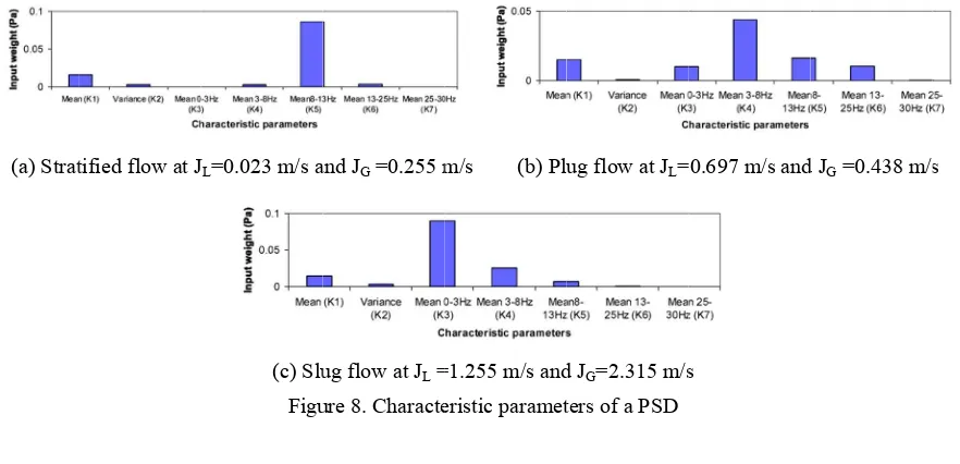
3.3.1 Char Based on t over 0-30 (2005). Th 0-30 (K2), (K7) use a
(a) Strat
(a) Typical of tim
Pattern Identif
racteristic Para the recorded p Hz is then di he mean value , mean 0-3 Hz as input of neur
tified flow at J
Time series si me series signal
fication Using
ameters of PSD power spectra, ivided into fiv e of power in (K3), mean 3 ral network tra
JL=0.023 m/s a
(c) Slu Figu
ignal l pressure grad
Back Propaga
D
this works fo ve bandwidths each of the a -8 Hz (K4), m aining.
and JG =0.255 m
ug flow at JL = ure 8. Characte
dient and PSD
ation Neural N
ocus on a frequ : 0-3, 3-8, 8-1 forementioned mean 8-13 Hz (
m/s (b) Plu
=1.255 m/s and eristic paramet
(b) Power in slug flow at
Networks
uency range up 13, 13-25, and d bands, denot (K5), mean
13-ug flow at JL=
d JG=2.315 m/s ters of a PSD
r spectral densi t JL=1.255 m/s
p to 30 Hz. Th d 25-30 Hz as ted as mean 0 -25 Hz (K6), a
=0.697 m/s and
s
ity
s and JG=2.315
he frequency r performed by 0-30 (K1), vari and mean 25-3
d JG =0.438 m/ 5 m/s
range y Xie iance 0 Hz
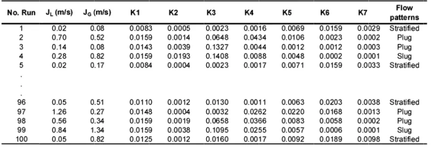
Table 2 sh operating flow) were
Table 2. E
3.3.2 Ident Neural net adding on train the n also get ne during trai generally i Back prop layer and componen three neura pipe (strat (0, 0, 1), th
Figu
hows part of condition. Tho e used to train
Examples of the
tifying Flow P tworks with a e or more/mul network to get etworking cap ining (but not it was begun b pagation neura one hidden nts of the inpu al cells, and co ified flow, plu hat of plug flow
ure 9. Back pro
characteristic ose parameter
the back propa
e vector charac
Pattern Using A single layer ha ltiple hidden l a balance the pabilities to pro
equal)). The by trying with o al network arch layer. The in ut vectors. The orresponds to ug flow and slu
w be (0, 1, 0),
opagation neural
parameters w rs and the outp agation ANN.
cteristic obtain
ANN ave a limitatio layers between
network's abil ovide the corr use of more t one hidden lay hitecture used nput layer co e hidden layer the three diffe ug flow). In th and that of slu
l network archit
with seven par put of the flow
ned from the pr
on in pattern re n input and ou lity to recogni rect response ( than one hidde yer.
d in the presen nsists of seve r consists of th erent flow patte his paper, let t ug flow be (1,
tecture is used in
rameter chara w patterns (str
resent study
ecognition. Th utput layers. B
ze patterns tha (with the inpu en layers have nt study is sho en neural cel hree neural ce erns of water-the expected o
0, 0).
n this research
acteristics of P ratified flow, p
his drawback c Back propagati
at will be used ut pattern is sim
e advantages f wn in Figure lls, correspond ells. The outpu
air two phase utput vector o
PSD for differ plug flow and
an be overcom ion neural net d during trainin
milar patterns for some cases 9. It has one ding to the s ut layer consis flows in horiz of stratified flo
rence slug
me by work ng. It used s, but input seven sts of
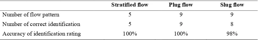
Table 3. P
art of test exam
red operating conditions are fication ability
Result of identi
f flow pattern f correct identi of identificatio
sion
r uses a differ eural network cteristics of th as the merits
his method ha tificial interve
ature
tificial neural n erential pressur
erage different rmalized press superficial ve uperficial veloc wer spectral de
edgments
k was supporte Education) M ascasarjana UG
e
Haluk, T., Jia ification in Air //dx.doi.org/10 H., & Beale, M
mples and iden
conditions of e selected as te
of the neural n
fication use Ba
ification as a advantag ntion.
network re (Pa) tial pressure (P
ure different s elocity (m/s)
city (m/s) ensity
ed by DP2M D Ministry of Edu
GM 2012”.
anhung, Q., & r-Water Two P 0.1002/cjce.545 M. (2000). Neur
ntification resu
f experiment a est samples. Ta network is very
ack Propagatio
Stratif
10
re transducer t dentifies the fl l pressure sign
computation ge method for
Pa) ignal (Pa)
DIKTI (Directo ucation and Cu
& John, S. A. Phase Flow. Th
50720308
ral Network To
ults
are selected as able 3 and Tab
y good.
on Artificial N
fied flow
5 5 00%
to measure th flow pattern. St
nals at differe and easily qu the industrial
orate of Resea ulture Indonesi
. (1994). Neu
The Canadian J
oolbox for Use
s training mod ble 4 show the
he differential tatistical analy ent flow cond uantifying the l application s
arch and Publi ia through the
ural Network
Journal of Che
e with MATLAB
dels to train th result of iden
ks
Slu
9
pressure of tw ysis of PSD w ditions. Result characteristic such as high
ic Service of D Competitive G
Based Object
emical Enginee
B. The MathW
he network an ntification, in w
ug flow
9 8 98%
wo phase flow as used to qua ts showed tha cs of the meas
accuracy, fast
Directorate Ge Grant Research
tive Flow Re
Drahos, J., Tihon, J., Serio, C., & Liibbert, A. (1996). Deterministic chaos analysis of pressure fluctuations in a horizontal pipe at intermittent flow regime. The Chemical Engineering Journal, 64, 149-156. http://dx.doi.org/10.1016/S0923-0467(96)03128-4
Drahos, J., Zahradnik, J., Puncochar, M., Fialova, M., & Bradka, F. (1991). Effect of operating conditions on the characteristics of pressure fluctuations in a bubble column. Chemical Engineering and Processing, 29, 107-115. http://dx.doi.org/10.1016/0255-2701(91)87019-Y
Ding, H., Zhiyao, H., Zhihuan, S., & Yong, Y. (2007). Hilbert–Huang transform based signal analysis for the characterization of gas–liquid two-phase flow. Flow Measurement and Instrumentation, 18, 37-46. http://dx.doi.org/10.1016/j.flowmeasinst.2006.12.004
Fausett, L. (1994). Fundamental of Neural Networks. Prentice Hill, New Jersy .
Jia, Z., Niu, G., & Wang, J. (2005). Identification of flow regimes in a horizontal flow using neural network.
Journal of Hydrodynamics, Ser. B, 17(1), 66-73, China Ocean Press.
Matsui, G., Fujino, G., & Suzuki, M. (2007). Two Phase Flow sensing using differential pressure fluctuations.
Jurnal of JSEM, 7, 50-55.
Wu, H., Zhou, F., & Wu, Y. (2001). Intelligent identification system of flow regime of oil-gas-water multiphase flow. International Journal of Multiphase Flow, 27(3), 459-475. http://dx.doi.org/10.1016/S0301-9322(00)00022-7
Xie, T., Ghiaasiaan, S. M., & Karrila, S. (2004). Artificial neural network approach for flow regime classification in gas-liquid-fiber flows based on frequency domain analysis of pressure signals. Chemical
Engineering Science, 59(11), 2241-2251. http://dx.doi.org/10.1016/j.ces.2004.02.017
Appendix
The PSD Theory
The goal of spectral analysis is to describe the distribution of the power contained in a signal over a frequency, based on a finite set of data. It converts information available in the time-domain into the frequency-domain. The averaged modified periodogram method was adopted to diminish the distortion of the spectrum due to a finite length of data record. If x(n) (n=0, 1, ... , N−1) is only measured over a finite interval, the power spectral density may be computed using the periodogram method:
k
fs f k i
e k x R f
Px( ) ˆ 2
(2)
Where: N is finite length of a discrete time signal, k is discrete time shift, f is frequency,fs is the sampling frequency and the autocorrelation is given as
N k
N n
n x k n x N k x R
1
) ( ) ( 1 ) ( ˆ
(3)
The Statistical Theory
The statistical analysis methods mentioned clustered PSD data are mean and variance. These features are used as inputs to the neural network.
The mean is given by,
N
i i
x
N 1
1
(4)
The variance is given as,
N
i i
x
N 1
2 1
1
(5)
These networks usually contain three types of layers: 1. An input layer
2. A hidden layer sigmoid bipolar and 3. An output layer linear transfer/ramp Training process:
Step 1. Design the structure of neural network and input parameters of the network Step 2. Get initial weights W and initial values from randomizing.
Step 3. Input training data matrix X and output matrix T. Step 4. Compute the output vector of each neural unit. (a) Compute the output vector H of the hidden layer
ik i k k W Xnet
(6)
k
k f net
H
(7) (b) Compute the output vector Y of the output layer
kj i j j W Hnet
(8)
j j f netY
(9) Step 5. Compute the distances
(a) Compute the distances d of the output layer
j j
jj T Y f'net
(10) (b) Compute the distances of the hidden layer
j
k kj
j
k W f' net
(11)
Step 6. Compute the modification of W and ( is the learning rate) (a) Compute the modification of W and of the output layer
k j kj H
W
(12) j
j
(13) (b) Compute the modification of W and of the hidden layer
i k
ik X
W
(14)
k k
(15) Step 7. Renew W and
(a) Renew W and of the output layer
kj kj kj W W
W
(16)
j j j
(17)
ik ik
ik W W
W
(18)
k k
k
(19) Step 8. Repeat step 3 to step7 until convergence.
Testing process:
Step 1. Input the parameters of the network. Step 2. Input the W and
Step 3. Input an unknown data matrix X Step 4. Compute the output vector
(a) Compute the output vector H of hidden layer
ik i k k W Xnet
(20)
k
k f net
H
(21) (b) Compute the output vector Y of the output layer
kj i j j W Hnet
(22)
j j f netY