LEAST SQUARES IMAGE MATCHING: A COMPARISON OF THE PERFORMANCE
OF ROBUST ESTIMATORS
Zeyu Li a,*, Jinling Wang b
a School of Civil and Environmental Engineering, University of New South Wales, Sydney, 2052,Australia – [email protected]
b
School of Civil and Environmental Engineering, University of New South Wales, Sydney, 2052,Australia – [email protected]
Commission VI, WG VI/4
KEY WORDS: Least Squares Image Matching, Robust Estimators, Accuracy, Comparison, Systematic errors, Outliers
ABSTRACT:
Least squares image matching (LSM) has been extensively applied and researched for high matching accuracy. However, it still suffers from some problems. Firstly, it needs the appropriate estimate of initial value. However, in practical applications, initial values may contain some biases from the inaccurate positions of keypoints. Such biases, if high enough, may lead to a divergent solution. If all the matching biases have exactly the same magnitude and direction, then they can be regarded as systematic errors. Secondly, malfunction of an imaging sensor may happen, which generates dead or stuck pixels on the image. This can be referred as outliers statistically. Because least squares estimation is well known for its inability to resist outliers, all these mentioned deviations from the model determined by LSM cause a matching failure. To solve these problems, with simulation data and real data, a series of experiments considering systematic errors and outliers are designed, and a variety of robust estimation methods including RANSAC-based method, M estimator, S estimator and MM estimator is applied and compared in LSM. In addition, an evaluation criterion directly related to the ground truth is proposed for performance comparison of these robust estimators. It is found that robust estimators show the robustness for these deviations compared with LSM. Among these the robust estimators, M and MM estimator have the best performances.
*
Corresponding author
1. INTRODUCTION
Image matching is an active research field in digital photogrammetry and computer vision. The main task in image matching is to find the corresponding pixel on two images of the same physical region. Usually the two images are referred as the reference image and the querying image respectively. In general, this is one fundamental step of various vision-based applications such as camera calibration, panorama generation, object recognition, structure from motion (SFM), 3D map generation and vision-based navigation.
Different matching methods such as keypoint matching and area-based matching are proposed by many researchers. Among them, least squares image matching (LSM) is still attractive for its definite mathematical description of the two patches and high accuracy. Moreover, quality control in the surveying domain can be implemented on LSM.
LSM’s creation can be traced back to the 1980s when Förstner (1982) firstly put forward the basic idea for LSM. Now the most widely used LSM utilises the intensity as the observation, and combines affine transformation model and linear radiometric model. Since it is a nonlinear model, Taylor linearization transfers the nonlinear model into the linear one to solve the unknowns through iterations. At the same time, because the number of observations exceeds that of unknowns, the solution can be obtained in a least squares sense. Finally, an accurate matching is acquired by the solution. Thus, LSM in essence is one process of nonlinear regression.
LSM has been widely researched and explored to enhance its adaptability and performance. For example, Bethmann and Luhmann (2011) employed the new projective transformation model in the functional model to improve the adaptability. In terms of the stochastic model, most researchers assumed that the measurements involved had equal precision and statistically independent, thus the weight matrix was a diagonal matrix. However, Wu et al. (2007) adapted the stochastic model by Blue estimator and the result showed that the new stochastic model improved matching accuracy by 0.2-0.4 pixel.
Acting as a matching refinement method, LSM has been extensively applied in different types of photogrammetric software. For example, Zhang et al. (2011) put forward a three-step scheme for keypoint matching on low-attitude images acquired by remotely piloted aerial vehicles. Pyramid-based LSM acted as the last step for refinement to improve the precision of keypoint matching. Ultimately a 3D city model was generated. Debella-Gilo and Kääb (2012) explored LSM’s application on surface displacement and deformation of mass movements, and showed that LSM could match the images and computed longitudinal strain rates, transverse strain rates and shear strain rates reliably and accurately.
distortions the quality of initial values, and the functional model.
This paper focuses on robust estimation to eliminate the influence of derivations from the LSM model. Two sources are presented. Firstly, the initial values of the unknowns are important since LSM is based on Taylor linearization. Keypoint matching is one method to obtain the initial values, but mismatches may happen. Therefore if the initial values of the unknowns are not close enough to the correct solution, the error caused by linearization will be large, resulting in a matching failure in the end. However, according to Baine and Rattan (2012), compared with their corresponding points in the reference image, if all the corresponding points in the querying image have a constant bias with the same magnitude and direction, the biases can be classified as systematic errors. Thus, this paper simulates this special case for LSM applications.
Secondly, another type of deviation—Salt & Pepper noise—is considered in this paper. It models the malfunction of the imaging sensor, and simulates other common conditions such as poor illumination, signal transmission and high temperature.
Since LSM already defines the model for the data, which means that the “normal” data pattern has been determined. If one set of data is “faraway” from the main part of the data, it can be identified as deviations. Generally, if the deviation is not large enough, there will be a tiny influence on the final result. However, if it is sizable, it can be identified as an outlier, causing masking and swamping effect, thus it will affect the final solution for linear or nonlinear estimations.
Multiple outliers rather than one single outlier are in existence with a higher possibility, and it is well known that the estimation in LSM is essentially least squares estimation, which is highly sensitive to outliers. Even though certain data pre-processing procedure has conducted outlier detection, it is much safer to involve outlier detection and exclusion in LSM. Statistically outlier detection in linear regression can be divided into two categories. One method is to detect and exclude the outliers based on some criterions such as Hadi potential (Hadi, 1992), elliptic norm (Cook and Weisberg, 1982) and Atkinson’s distance (Anscombe, 1963). These methods are originally designed for detecting the single outlier. However, under certain circumstance, it can be used iteratively to remove multiple outliers. Another method is robust estimation which involves all the observations but reduce the influence of underlying outliers. In this paper, varieties of robust estimators, such as M estimator and S estimator, replace the traditional estimation method (least squares estimation) in LSM, and are compared in terms of the success rate, which is one measurement for all the simulated corresponding points.
There have been extensive studies concerning the comparison on different robust estimators. Knight and Wang (2009) made the comparison of robust estimators on simulated GPS measurements in terms of the ability of outlier exclusion. They demonstrated that no method could correctly exclude all the outliers. For the single outlier, the highest performance is obtained by MM estimator and L1-norm. Ge et al (2013) made the comparison of 13 commonly used robust estimation methods in the GPS coordinate transformation of the four- and seven-parameter models. With the simulated experiment which controls the different coincident points and the number of gross errors, they showed that L1 and German-McClure method are relatively more efficient.
To the best of our knowledge, the comparison of robust estimator under the situation of systematic errors and outliers for LSM has not been analysed. Therefore, it is the focus of this paper. The rest of this paper is organized as follows. The brief introduction of LSM is presented in Section 2, and the description of outlier sources is proposed in Section 3. Concerning this issue, we introduce robust estimators in Section 4, and then details about the preparation of real data and simulation data are described in Section 5. Section 6 shows the experimental result and related analysis for comparison. Finally, the concluding remarks in Section 7 summarize the outcome of the experiment and describe possible directions of research of LSM in the future.
2. LEAST SQUARES IMAGES MATCHING Although LSM has been improved in terms of the functional model and the stochastic model for better performance and adaptability, the most common LSM will be briefly introduced in this section as the foundation for further discussions in this paper.
As an area-based matching method, LSM firstly defines the relationship between two patches with the same size in two images. It takes advantage of the affine transformation model to describe the geometry and the linear model to describe the intensity variation as shown in (1).
(1)
where , = the intensity of the reference image and the querying image respectively. They all depend on the image coordinate and
= the unknowns in the affine transformation model
= the unknowns in the linear model of intensity
However, the solution cannot be acquired directly since it is a nonlinear function. Therefore with the help of Taylor linearization, it is transformed to a linear one as illustrated in (2).
(2)
The intensity and coordinates of all corresponding pixels from the two patches are grouped together in the form of (2). Hence a design matrix and its corresponding observations are formed. Generally the number of observations exceeds the undetermined parameters. Thus, traditionally the unknowns can be solved by least squares estimation. Finally the iterative process is applied to acquire the final results. However, the iteration needs the terminating criterion, which is usually judged by correlation coefficient between the two patches, or the norm of the corrections is less than a certain small threshold.
3. SOURCES OF DEVIATIONS IN LSM
according to Taylor linearization based on the intensity in the patch, cannot appropriately fit the model determined by LSM, LSM will not converge to a correct solution, causing mismatches in the end.
To figure out the reason why sometimes LSM work properly n some cases, to the best of our knowledge, the two kinds of sources, which are systematic errors and outliers, are presented and analysed in this section
3.1 Systematic Errors (Initial Bias)
As noted above, LSM is essentially based on Taylor linearization, which needs the appropriate estimation on the initial value of the solution. In other words, the initial values have to be close enough to the solution. One method to acquire the initial value of unknowns is keypoints matching and extraction such as SURF (Bay et al., 2006) and BRISK (Leutenegger et al., 2011). Therefore, to obtain the parameter in the affine transformation model, the tentative keypoints need to be matched as accurately as possible.
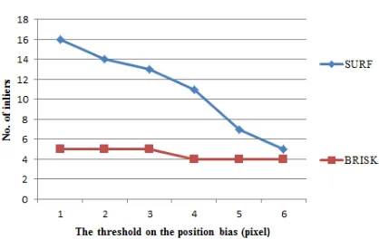
However, for the practical situation such as the commonly used method RANSAC, when the keypoints are extracted and matched before going through RANSAC with the affine transformation model, they still have re-projection errors which are the basis for setting the threshold of inliers and outliers. Although the error can be controlled with a stricter threshold, it still faces the shortage of available corresponding keypoints in certain circumstances. For example, in the following stereo images pair A and B taken from UAV (Figure 1), SURF and BRISK points are extracted and matched, then filtered by RANSAC. If the threshold is set from 1 pixel to 6 pixels, the number of the available keypoints shows a decreasing trend as demonstrated in Figure 3. At the same time, it is an example of the existence of initial bias on image matching.
(a) The image A (b) The image B
Figure 1. The stereo images taken by a UAV
Figure 2. The variation on the number of inliers with different thresholds
If all the biases of the keypoints position have the same magnitude and direction, it denotes the systematic error, which is considered by the simulation in Section 5.
3.2 Outliers (Imaging Sensor Malfunction)
This relates to faults in the imaging sensor. A few pixels in the COMS or CCD sensor will not function properly, commonly resulting in dead or stuck pixels on the generated image. However, this rarely happens to the professional photogrammetric cameras since they are strictly tested and excluded by the manufacturer. Nevertheless, in terms of consumer-level cameras, a limited number of pixels (usually 3 at most for the entire pixels of the sensor) are allowed to exist in by the manufacturer considering the cost. Thus, this will also lead to the error on the observation (intensity) in LSM though the chances are very low. These high-leverage pixels statistically can be identified as outliers.
The imaging sensor malfunction can be modified as Salt & pepper noise, which is illustrated in (3).
{
(3)
where = the intensity of the noise-free image = the intensity of the image with noises = the percentage of affected pixels
Usually the traditional method to deal with this kind of noise is to denoise the contaminated image with various filters such as Mean filter, Gaussian filter and so on (Bovik, 2005). However, in this paper, the influence of noise is reduced from the perspective of data processing and optimal estimation. Salt & Pepper noise acts as the noise model when there are faults in the imaging sensor, thus least squares estimation is heavily affected and cannot be optimal. Thus the robust estimators are introduced in the next section.
4. ROBUST ESTIMATION
Since LSM possibly involve deviations from various sources as mentioned above, it is highly necessary to control the influence of deviations. In this section, we will briefly introduce four categories of robust estimation method: RANSAC-based method, M estimator (Reweighting-based method), S estimator and MM estimator.
Two metrics that describe the robustness and precision of estimators are breakdown point and relative efficiency. Among these estimators, least median of squares (LMedS) estimator, S estimator and MM estimator have high breakdown point of 0.5, which means that they can tolerate up to 50% outliers. Besides, M estimator’s robustness is related to the selection of weight function, and least absolute deviations (LAD) has zero breakdown point. For relative efficiency, M and MM estimator have the higher efficiency of 95%, while LAD estimator, LMedS and S estimator have relative efficiency of 64%, 37% and 33% respectively.
4.1 Ransac-based Methods
sum of absolute standardized residuals. There are a number of methods to find the minimum of the two objective functions. However, RANSAC is applied to research the entire data and obtain the solution.
(4)
∑| |
(5)
where = the standardized residual
An important parameter for RANSAC is the percentage of outliers or the inliers, which define the minimum number of iterations for the given success rate, which is shown in (6). In this paper, the percentage of inliers is assumed to be 0.5. Besides, and are set to be 0.95 and 8 respectively.
(6)
where = the success rate of RANSAC = the percentage of inliers
= the number of observations to solve the unknowns
4.2 M Estimator (Reweighting-based Method)
M estimator is another common method for robust estimation with the advantage of high efficiency. Instead of minimizing∑ , these reweighting-based M estimators tries to minimize ∑ , where is less increasing than the square function in least squares estimation, and it is a symmetric, positive-define function with only one unique minimum at zero. However, in practice, we make use of the weighting functions, which is the second derivative of . The detailed derivation can be found in the book of James (2005). The following equations are the weighting functions for standardized residuals. All and in the following equations represent the standardized residuals of the least squares solution and the turning value respectively from other searcher’s recommendation.
(a) Huber Method (Huber, 1981)
{ | | | | (7)
(b) Andrews Method (Andrews, 1974)
{
| | | |
| | ( (8)
(c) Welsch Method (Holland and Welsch, 1977)
{
| | | |
| | ( (9)
(d) Fair Method (William, 1983)
| | ( (10)
(e) Cauchy Method
| | ( (11)
4.3 S Estimator
One characteristic of S estimator is high breakdown point. It tries to minimise the dispersion of the residuals. According to Rousseeuw and Leroy (1987), it tries to find , which is the dispersion of residuals, as the solution of (12)
∑ (12)
where is a constant defined as with having a standard normal distribution, and satisfies
. Besides, is a appreciate function which is symmetric, continuously differentiable, strictly increasing on and constant on
.
Since S estimator is computationally expensive, S estimator with Fast-S algorithm is applied in this paper. Its detailed process can be found in Salibian-Barrera and Yohai (2006).
4.4 MM Estimator
MM (Yohai, 1987) estimator makes use of S estimator to obtain the initial estimate, and the residuals acquired from S estimator can be used to determine the scale factor of M estimator. With the scale factor, an iteratively reweighted least squares procedure like that of M estimator is implemented to acquire the final solution. MM estimator has the property of high breakdown point and high efficiency. In this paper, to reduce the computational burden, Fast S (Salibian-Barrera and Yohai, 2006) estimator is applied for the initial estimate.
5. TEST DESIGN
In the following experiments, both simulation data and real data are tested to compare the robust estimators’ performance. To reduce the bias and ensure test adequacy, seven images including 3389 patch pairs are generated and tested. This section describes the generation and selection of simulation data and real data for LSM.
5.1 Simulation Data Preparation
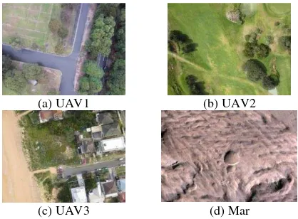
The convergence of LSM is related to image texture, which is hard to be controlled. Therefore this paper presents a set of images for different environments to reduce the bias of the testing data. They are three images taken by a low altitude UAV, and one image of Mars surface coming from NASA's Mars Reconnaissance Orbiter (MRO), which are all listed sequentially in Figure 3.
(a) UAV1 (b) UAV2
(c) UAV3 (d) Mar
Figure 3. The reference images for simulation
To generate the simulated corresponding point in the reference image, four nets consisting of such points are created with different intervals. The numbers of simulated corresponding points for the four images are different since the images have different width and length except the image 2 and 3. The detailed information about the four images is shown in Table 1.
UAV1 UAV2 UAV3 Mars
No. of Points 450 609 609 486
Resolution Ratio 4000×3000 4608×3456 4608×3456 1413×951
Table 1. The characteristics of the simulated image pairs
For the generation of “simulated” points in the querying image, a special affine transformation model following (13) is applied, which is
(
) (13)
Actually the simulation degenerates to a translation model that avoids scaling and rotational variation. Besides, there are no occlusions in the simulated querying image. It should be noted that this is often the case for the epipolar image, which is commonly used for stereo matching and digital elevation model (DSM) generation. Besides, the epipolar image can be generated from non-epipolar image by image rectification, such as the images from Middlebury Stereo Datasets.
Figure 4. The image 1 (the reference image) and its simulated image (the querying image)
Finally, four image pairs are produced from the four testing images. For instance, as show in the Figure 4, there is a 20-pixel-wide strip in its simulated image, which means that all the simulated points are translated towards the right direction for 20 pixels.
It should be noted that a terminating criterion is applied in the iteration of LSM in the simulation experiment. That is when the
parameters in the affine transformation model lead to the overflow from the boundary. This means that LSM has already failed.
To evaluate the accuracy of the final result from LSM, the final corresponding coordinates of the simulated points are employed from LSM instead of checking correlation coefficient, since a higher correlation coefficient does not necessarily reflect the higher matching accuracy, therefore, according to the affine transformation model in (13), the final accuracy can be calculated by using (14).
√ (14)
where and are the final coordinate of the simulated corresponding points on the reference image and querying image from LSM respectively. Subscript and represent reference images and querying images. If the value obtained from (14) is less than 0.001 pixel, it is counted as an accurate matching pair. Besides, we count the number of tentative matching pairs that pass the terminating criterion, if the total number of accurate matching pair, which is the number of matching pair that passed (14) divided by the total number of tentative matching pair, a ratio can be acquired. This means the success rate for LSM.
5.2 Real Data Preparation
Three image pairs from Middlebury Stereo Datasets (Scharstein and Szeliski, 2003) that involve occlusion and changes of view are selected for LSM, which are listed in Figure 5, and the details of image are shown in Table 2.
(a) Baby (b) Aloe (c) Cloth
Figure 5. The reference images from Middlebury
Baby Aloe Cloth
No. of Points 399 418 418
Resolution Ratio 1110×1240 1110×1282 1110×1282
Table 2. The characteristics of the real image pairs
The corresponding point net is generated following the same procedure of simulation data preparation for each reference image. However, since each image pair has its ground truth disparity image with accuracy 1 pixel, the calculation of final accuracy is changed to (15) accordingly, which is:
√ (15)
where is the disparity of corresponding point pairs. In addition, since LSM can obtain sub-pixel level accuracy, the criterion for the success rate is changed to 1 pixel accordingly. Moreover, in the experiments on both simulation data and real data, the size of the patch is pixels and the maximum number of iterations is 10.
Images
Trait
6. TEST RESULT AND ANALYSIS 6.1 Test Result on Simulation Data and Analysis
Four different noise levels, which are the percentages of malfunctioning pixels on the imaging sensor, are set at 0%, 0.1%, 0.5% and 1% respectively on simulation data. Therefore, four scenarios are generated. Systematic error (SE) from 0.5 pixel to 3 pixels are added on the simulated corresponding points in first scenario without noise, However, because of the noise and the higher criterion (0.001 pixel) for the success rate, OLS seldom work well, therefore the systematic error is set from 0.5 pixel to 1.5 pixels in the remaining ones, and more extreme conditions with a higher noise level are not tested. For a better illustration, all the simulated corresponding points from the four images are added together as a whole to evaluate the overall performance of various robust estimators under different noise levels. The results from different estimators are shown in Table 3-6.
It can be illustrated from the results that with the increase of systematic errors, the success rates of all the estimation methods generally have decreasing trends, However, it is interesting to find that the success rate slightly increases when the systematic error changes from 0.5 pixel to 1 pixel on M estimator in Table 6, which shows the robust estimators’ resistance for outliers
When the systematic error is around 1 pixel without noise, OLS can maintain the success rate at nearly 100% for the simulation data. Nevertheless, when the systematic error increases to 3 pixels, OLS can hardly keep up the success rate as it is heavily influenced by the deviation from the model of LSM. However, at the same time, other robust estimators show the robustness in dealing with the systematic error compared with OLS. When the noise is injected in the simulation data, OLS is further affected. Moreover, other robust estimators continue to show the resistance for outliers.
The performance of four categories of robust estimators can also be demonstrated by the results. The performances of RANSAC-based methods are unstable and lower compared with other estimators. Especially when the systematic error is higher with noise level 0% and 0.1%, they even cannot compete with OLS.
0. 5 pixel
1 pixel
1.5 pixels
2 pixels
2.5 pixels
3 pixels
OLS 99.07% 99.44% 97.82% 76.93% 69.36% 50.00%
LMedS 82.17% 75.63% 64.72% 33.66% 24.09% 5.34%
LAD 71.03% 64.53% 53.25% 28.00% 18.66% 7.99%
Huber 99.44% 99.81% 98.23% 80.41% 74.00% 55.16% Andrews 99.17% 99.40% 98.00% 80.18% 73.16% 54.97%
Welsh 99.35% 99.68% 98.14% 80.78% 74.19% 56.26% Fair 99.40% 99.81% 98.37% 80.64% 74.00% 55.52% Cauthy 99.26% 99.77% 98.38% 80.64% 74.32% 56.27% FastS 95.41% 95.45% 92.48% 73.49% 63.00% 41.92%
MM 98.84% 99.16% 97.54% 80.04% 73.49% 55.44%
Table 3. The success rate on simulation data with noise level 0%
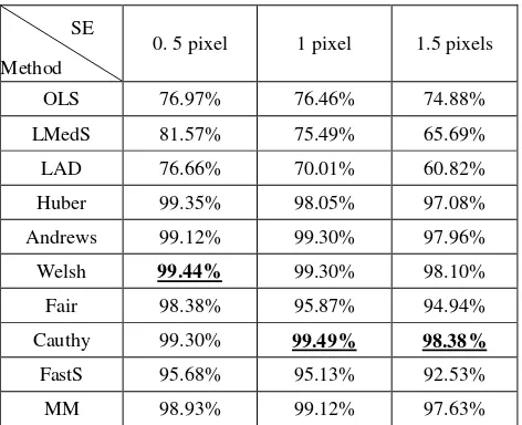
0. 5 pixel 1 pixel 1.5 pixels
OLS 76.97% 76.46% 74.88%
LMedS 81.57% 75.49% 65.69%
LAD 76.66% 70.01% 60.82%
Huber 99.35% 98.05% 97.08%
Andrews 99.12% 99.30% 97.96%
Welsh 99.44% 99.30% 98.10%
Fair 98.38% 95.87% 94.94%
Cauthy 99.30% 99.49% 98.38%
FastS 95.68% 95.13% 92.53%
MM 98.93% 99.12% 97.63%
Table 4. The success rate on simulation data with noise level 0.1%
0.5 pixel 1 pixel 1.5 pixels
OLS 27.21% 25.63% 24.98%
LMedS 81.34% 75.30% 66.16%
LAD 75.12% 67.73% 56.04%
Huber 94.66% 86.54% 86.77%
Andrews 97.96% 96.84% 95.73%
Welsh 98.42% 96.05% 95.64%
Fair 89.60% 77.76% 77.16%
Cauthy 97.31% 94.29% 92.99%
FastS 95.17% 95.59% 92.71%
MM 98.93% 99.03% 97.45%
Table 5. The success rate on simulation data with noise level 0.5%
0.5 pixel 1 pixel 1.5 pixels
OLS 7.61% 6.69% 6.31%
LMedS 81.38% 74.56% 63.51%
LAD 67.87% 57.29% 46.33%
Huber 81.57% 66.48% 67.04%
Andrews 94.71% 89.00% 89.83%
Welsh 89.14% 80.55% 80.22%
Fair 72.10% 56.04% 56.17%
Cauthy 89.88% 81.75% 81.34%
FastS 95.68% 94.71% 93.18%
MM 98.75% 98.38% 96.84%
Table 6. The success rate on simulation data with noise level 1%
The result from Fast S estimator is also not stable. In the scenario without noise, it has a lower performance than OLS. SE
Method
Method SE
Method SE
However, when the noise is injected into the simulation data, Fast S estimator has a competitive performance with MM estimator especially when the noise level is 1%. RANSAC-based methods and Fast S estimator’s performance is unsatisfactory in the scenario without noise. One possible reason is that they wrongly eliminate the influence of some good observations fitting the model.
When the noise level is 0 and 0.1%, M estimators perform the best although their advantages are not obvious. However, when the noise level increases to 0.5% and 1%, MM estimator outperforms other estimators considerably.
6.2 Test Result on Real Data and Analysis
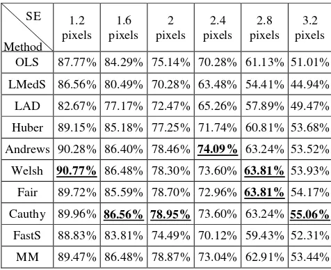
The test on the real data basically follows the same procedure of simulation data. However, the interval of systematic error is replaced by 0.4 pixel. The results from different estimators are shown in Table 7-10.
The results of the real data basically show the consistent performances of robust estimators with that of simulation data, but they still have certain differences.
1.2
Table 7. The success rate on real data with noise level 0%
1.2
Table 8. The success rate on real data with noise level 0.1%
1.2 Table 9. The success rate on real data with noise level 0.5%
1.2 Table 10. The success rate on real data with noise level 1%
Overall, the same estimators have lower success rates compared with the simulation data. This is because the real data includes the factors that are more likely to exist in the real practice such as the change of view and occlusion.
The criterion of success rate for the real data is lower than that of simulation data as the accuracy of ground truth is 1 pixel, therefore when the systematic error is up to 3.2 pixels in the presence of noise, the success rate can be higher than that of the simulation data.
RANSAC-based methods outperform OLS when the noise level is 0.5% and 1%. However, when the noise level is lower, their success rates are slightly lower than OLS and other estimators except in some cases when the noise level is 1%.
the noise level, MM perform the best among all the other estimators.
7. CONCLUDING REMARKS
With both simulation data and real data, four categories of robust estimation method including RANSAC-based method, M estimator, S estimator and MM estimator are applied and compared as the estimation method in LSM. Therefore some concluding remarks can be made. Firstly, it is found that systematic error (initial bias) on LSM should be controlled within 1.5 pixels to maintain the high performance. Secondly M and MM estimators have the higher ability to eliminate the influence of deviations compared with other estimators, thus when both systematic error and image quality are unknown, the two robust estimators provide a comparative and safe alternative of OLS method in LSM.
To linearize a nonlinear function for parameter estimation, the convergence also has the relationship with the function itself. Similarly, the model determined by LSM is a function about the intensity that depends on the image coordinate and , and other related coefficients, which directly comes from the texture of the image. However, if the nonlinearity of the model in LSM does not allow the linearization, LSM will not converge to a correct solution. But how nonlinearity of the function is linked with the image texture remains a problem that needs to be further explored.
ACKNOWLEDGEMENTS
The first author is sponsored by China Scholarship Council (CSC) for his PhD studies at UNSW Australia. Sincerely thanks go to Dr. Yincai Zhou and Dichen Liu for providing the UAV images, as well as Joossens K for providing the related Matlab function.
REFERENCES
Andrews, D. F., 1974. A robust method for multiple linear regression. Technometrics, 16(4), pp. 523-531.
Anscombe, F. J., Tukey, J. W., 1963. The examination and analysis of residuals. Technometrics, 5(2), pp. 141-160.
Baine, N. A., Rattan, K. S., 2012. Algorithm for the detection and isolation of systemic measurement errors in vision based/aided navigation systems. In: 2012 IEEE/ION Position, Location and Navigation Symposium, Myrtle Beach, SC, USA, pp. 366-370.
Bay, H., Tuytelaars, T., Van Gool, L., 2006. Surf: Speeded up robust features. In: 2006 European Conference on Computer Vision, pp. 404-417.
Bethmann, F., Luhmann, T., 2011. Least-squares matching with advanced geometric transformation models. Photogrammetrie-Fernerkundung-Geoinformation, 2011(2), pp. 57-69.
Bovik, A. C., 2005. Handbook of Image and Video Processing. Elsevier Academic Press.
Cook, R. D., Weisberg, S. 1982. Residuals and Influence in Regression. CHAPMAN and HALL.
Debella-Gilo, M., Kääb, A., 2012. Measurement of surface displacement and deformation of mass movements using least squares matching of repeat high resolution satellite and aerial images. Remote Sensing, 4(1), pp. 43-67.
Förstner, W., 1982. On the geometric precision of digital correlation. International Archives of Photogrammetry and Remote Sensing, 24(3), pp. 176-189.
Ge, Y., Yuan, Y., Jia, N., 2013. More efficient methods among commonly used robust estimation methods for GPS coordinate transformation. Survey Review, 45(330), pp. 229-234.
Hadi, A. S., 1992. A new measure of overall potential influence in linear regression. Computational Statistics & Data Analysis, 14(1), pp. 1-27.
Holland, P. W., Welsch R. E., 1977. Robust regression using iteratively reweighted least-squares. Communications in Statistics: Theory and Methods, pp. 813–827.
Huber, P. J., 1981. Robust Statistics. John Wiley, New York.
Knight, N. L., Wang, J., 2009. A comparison of outlier detection procedures and robust estimation methods in GPS positioning. Journal of Navigation, 62(04), pp. 699-709.
Leutenegger, S., Chli, M., Siegwart, R. Y., 2011. BRISK: Binary robust invariant scalable keypoints. In: 2011 IEEE International Conference on Computer Vision, pp. 2548-2555.
Powell, J. L., 1984. Least absolute deviations estimation for the censored regression model. Journal of Econometrics, 25(3), pp. 303-325.
Rousseeuw, P. J., 1984. Least median of squares regression. Journal of the American Statistical Association, 79(388), pp. 871-880.
Rousseeuw, P. J., Leroy, A. M., 1987. Robust Regression and Outlier Detection. Wiley, Hoboken.
Salibian-Barrera, M., Yohai, V. J., 2006. A fast algorithm for S-regression estimates. Journal of Computational and Graphical Statistics, 15(2).
Scharstein, D., Szeliski, R., 2003. High-accuracy stereo depth maps using structured light. In: IEEE Computer Society Conference on Computer Vision and Pattern Recognition (CVPR 2003), Madison, WI, USA, 1, pp. 195-202.
William, J. J. R., 1983. Introduction to Robust and Quasi-Robust Statistical Methods. Springer, Berlin.
Wu, J., Zhang, Q., Wang, J., 2007. Least squares image matching and precision improvement. Journal of Photogrammetry and Remote Sensing, 12(3), pp. 217-224.
Yohai, V. J., 1987. High breakdown point and high efficiency robust estimates for regression. The Annals of Statistics, 15, pp. 642–656.