Directory UMM :Data Elmu:jurnal:J-a:Journal of Empirical Finance (New):Vol7.Issue3-4.2000:

(1)

www.elsevier.comrlocatereconbase

Volatility dynamics under

duration-dependent mixing

John M. Maheu

a,)

_{, Thomas H. McCurdy}

b

a ₍ ₎

Department of Economics, UniÕersity of Alberta, Edmonton, AB, T6G 2H4 Canada b

Rotman School of Management, UniÕersity of Toronto, Toronto, ON, Canada

Abstract

This paper proposes a discrete-state stochastic volatility model with duration-dependent mixing. The latter is directed by a high-order Markov chain with a sparse transition matrix.

Ž .

As in the standard first-order Markov switching MS model, this structure can capture turning points and shifts in volatility, due for example, to policy changes or news events.

Ž .

However, the duration-dependent Markov switching model DDMS can also exploit the persistence associated with volatility clustering. To evaluate the contribution of duration

Ž .

dependence, we compare with a benchmark Markov switching-ARCH MS-ARCH model. The empirical distribution generated by our proposed structure is assessed using interval forecasts and density forecasts. Implications for areas of the distribution relevant to risk management are also assessed.q_{2000 Elsevier Science B.V. All rights reserved.}

1. Introduction

To manage risk associated with uncertain outcomes, one relies on forecasts of

Ž .

the distribution of k-period-ahead returns. The popular value-at-risk VaR calcu-lation of the loss that could occur with a specified confidence level over a given holding period focuses on a single quantile of that forecasted distribution. There

)_{Corresponding author. Tel.:}_q_{1-780-492-2049.}

Ž .

E-mail addresses: john.maheu@ualberta.ca J.M. Maheu , tmccurdy@mgmt.utoronto.ca

ŽT.H. McCurdy ..

Ž .

(2)

are several potential questions that would interest risk managers. Firstly, are the VaR numbers correct on average, or more generally, is the maintained uncondi-tional distribution adequate? Secondly, given available information, does one obtain accurate VaR numbers at each point of time? In other words, is the maintained conditional distribution adequate? Finally, if the answer to either of these questions is no, how might the risk manager’s model be improved? Implicit in these questions are difficult issues related to evaluation of the adequacy of alternative models, and the correct specification of the conditional and uncondi-tional distribution of returns.

Ž .

A first step to forecasting the distribution or some region thereof of future returns, is to investigate stylized facts concerning the statistical properties of returns for the asset or portfolio in question. Short-run price dynamics in financial markets generally exhibit heteroskedasticity and leptokurtosis. For the case of log price changes in foreign exchange markets, which is the application in this paper, there is also some evidence of convergence to a Gaussian distribution under time aggregation.1

The next step might be to postulate a probability model which can replicate such stylized facts. Since short-run returns are not IID, attention to the conditional density is warranted. One needs to postulate and estimate a probability model for the law of motion of returns over time. For currencies at weekly frequencies, strong volatility dependence combined with largely serially uncorrelated returns suggests that, for modeling purposes, the main focus should be on the conditional volatility dynamics. Volatility clustering implies predictability in the conditional variances and covariances. This empirical fact should contribute to risk manage-ment strategies.

In this paper, we concentrate on the choice of conditional volatility dynamics and ask what features a particular specification can deliver in terms of the conditional and unconditional distributions. We propose a model that emphasizes discrete changes in the level of volatility and introduces duration dependence to accommodate volatility clustering. The features of this model are compared with two benchmark models that do not include the duration structure. Of interest is whether a particular specification can simultaneously capture important properties in the conditional and the unconditional distributions.

Alternative models have been proposed to capture and forecast time-varying

Ž .

volatility for financial returns. For example, the generalized ARCH GARCH

Ž .

class Engle, 1982; Bollerslev, 1986 is based on an ARMA function of past innovations. These models have become the workhorse for parameterizing

in-1

There are many papers which report stylized facts for exchange rates, including Boothe and

Ž . Ž . Ž . Ž .

Glassman 1987 , Diebold 1988 , Engle and Hamilton 1990 , Hsieh 1989 , Kaehler and Marnet

(3)

tertemporal dependence in the conditional variance of speculative returns.2 Markov

Ž .

switching MS models for mixture distributions in which draws for component

Ž .

distributions follow a first-order Markov chain Lindgren, 1978; Hamilton, 1988 have also been applied to volatility dynamics.3Although such discrete-mixtures

Ž

models can generate most of the stylized facts of daily returns series Ryden et al.,

´

. Ž

1998 , there is some evidence for example, Hamilton, 1988; Pagan and Schwert,

.

1990 that the first-order Markov model with constant transition probabilities is inadequate with respect to capturing all of the volatility dependence.

This paper provides an alternative to the switching ARCH model introduced by

Ž . Ž .

Cai 1994 and Hamilton and Susmel 1994 . Our alternative approach is a discrete-state stochastic volatility model which incorporates a parsimonious high-order Markov chain to allow for duration dependence. As in the standard first-order MS model, this structure is useful for capturing shifts and turning points in volatility that are difficult to accommodate with the ARMA structure implicit in GARCH. However, unlike the standard model, a duration-dependent Markov

Ž . Ž

switching DDMS model Durland and McCurdy, 1994; Maheu and McCurdy,

.

2000; Lam, 1997 is particularly suited to exploiting the persistence associated with volatility clustering. This is achieved by several important features of our specification. Firstly, the duration variable provides a parsimonious parameteriza-tion of potential high-order dependence. Secondly, unlike the GARCH case, persistence is permitted to be time-varying by allowing the duration of a state to affect the transition probabilities. Thirdly, including duration as a conditioning variable in the conditional variance specification allows the model to capture a broad range of volatility levels.

MS models generate mixtures of distributions. These models can be motivated from information flows into the market. The application in this paper is to log-differences in foreign exchange rates. Exchange rates are good candidates for mixture models because an exchange rate is a relative price, which will be influenced by policy changes and news arrivals. News theories of price changes attribute an important role to the current innovation. In this case, a stochastic

Ž .

volatility SV component may be an important addition to time-varying but deterministic representations of volatility as in GARCH. The DDMS model is a discrete-time, discrete-state, SV model. Therefore, our approach provides a straightforward method of obtaining maximum likelihood estimates for SV with the added features discussed above.

Like standard first-order MS models, and other time-dependent discrete-mixture models, we model the stochastic process governing a switch from one volatility

2 _Ž _.

See, for example, a recent survey by Palm 1996 and references therein.

3 _Ž _. _Ž _. _Ž _.

For example, see Pagan and Schwert 1990 , Kaehler and Marnet 1993 , Klaassen 1998 , Kim et

Ž . Ž . Ž .

(4)

state to another. Incorporating the possibility of a discrete change in the level of volatility can have a substantial effect on the implied conditional and uncondi-tional distributions. This may contribute to an improved fit, particularly with respect to the tails of the distribution. Further, unlike standard MS models, allowing the transition probabilities to be duration-dependent may improve the model’s ability to capture intertemporal dependence. In addition, our approach models the evolution of volatility within each state. The DDMS model considered in this study is only a two-state model, however, it acts like a large N state model in that it can capture a broad range of volatility levels through conditioning on duration in the conditional variance.

In Section 2, we discuss the data and associated descriptive statistics. Section 3 summarizes the candidate models for volatility dynamics compared in this paper. Particular emphasis is applied to comparing the stochastic properties inherent in the forecasts implied by each. This is followed by model estimates in Section 4. Adequacy of the conditional distributions implied by those estimates is reported in

Ž

Section 5. For these assessments, we apply both interval forecasts Christoffersen,

. Ž .

1998 and density forecasts Diebold et al., 1998; Berkowitz, 1999 . In Section 6, we use simulation methods to investigate the properties of the unconditional distributions implied by the estimates of the alternative volatility models. Finally, Section 7 provides a brief summary of the features of the data that are matched by our alternative parameterizations.

2. Data and descriptive statistics

Let e denote the spot price in units of foreign currency for US$1. In this paper,_t

Ž . Ž

we report results for the Deutsche mark DEM-USD , and British pound

GBP-.

USD . Define y as the scaled log-difference of e , or the continuously com-_t _t pounded percentage return from holding a US$1-equivalent of foreign currency for a week,

et

yts100log .

Ž

2.1

.

ety1

4

Information available to the econometrician at time t is Vts y , yt ty1, . . . . Sample size is Ts1304, covering the time period from 1974r01r02 to 1998r12r23.

(5)

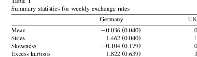
Table 1

Summary statistics for weekly exchange rates

Germany UK

Excess kurtosis 1.822 0.639 3.579 0.843

Ž . w x w x

Modified Q 1 1.157 0.282 1.472 0.225

Ž . w x w x

Modified Q 2 4.378 0.112 1.476 0.478

Ž . w x w x

Modified Q 10 11.320 0.333 11.565 0.315

2_Ž _. _w _x _w _x

Q 10 83.349 0.000 156.416 0.000

The data are percentage returns from weekly exchange rates with the US dollar from 1974r01r02 to 1998r12r23. Standard errors robust to heteroskedasticity are in parenthesis, p-values in square

Ž . 2_{Ž .}

brackets. Q j is the Ljung-Box statistic for serial correlation in the demeaned series, and Q j is the

Ž .

same in the squared series with j lags. The modified Q j allows for conditional heteroskedasticity

Ž .

and follows West and Cho 1995 .

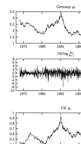
significant serial dependence associated with squared returns. Fig. 1 plots the levels e and log price changes y for the two currencies._t _t

3. Alternative parameterizations of volatility

In this section, alternative parameterizations of conditional volatility are dis-cussed. As a reference point, we begin by briefly summarizing the popular ARCH

Ž .

and a Markov switching-ARCH model MS-ARCH . Then duration dependence is

Ž .

introduced in a discrete-state parameterization of volatility the DDMS model by allowing the conditional transition probabilities, as well as the state-specific levels of volatility, to be functions of duration. The final subsection discusses some salient differences between the alternative parameterizations. In particular, we emphasize the potential impact of the duration-dependent components on volatility dynamics and forecasts.

3.1. GARCH

To introduce our discussion of alternative parameterizations of volatility,

Ž . 4

consider the popular GARCH 1,1 , which is defined as

s2_s_v_q_ae2 _q_bs2

_Ž

_3.1

_.

t t ty1 ty1

etsstz ,t zt;N 0,1

Ž

.

Ž

3.2

.

4

(6)

Fig. 1. Time series of exchange rates.

wheree_t is the innovation to the process y parameterized as,_t

(7)

For the purpose of residual-based diagnostic tests, the standardized residuals are formed using estimates of etrst.

Note that, except for the non-negativity constraint on s2

, volatility is a t

continuous variable. Also, in this formulation, conditional volatilitys2

is time-t

varying but deterministic, given the information set V_t_y₁. As the acronym ARCH implies, this model parameterizes volatility as autoregressive conditional het-eroskedasticity. In other words, it allows volatility clustering.

Ž .

A re-arrangement of Eq. 3.1 implies squared innovations follow an ARMA model, as in,

1yaLybL e2_s_v_q ₁_y_b_L _e2_y_s2 _,

Ž

.

t

Ž

.

Ž

t t

.

where L is the lag operator. Therefore, many of the properties of the stationary ARMA model, such as exponential decay rates, are imposed by this GARCH model on the squared innovations for returns. Furthermore, ARMA models are not

Ž .

well-suited to capturing discrete jumps up or down in volatility. This potential

Ž .

shortcoming of the plain vanilla GARCH parameterization in Eq. 3.1 is one of the motivations for exploring alternative models that can capture discrete regime changes in volatility.

3.2. MS-ARCH

One possibility is to combine an ARCH specification with a discrete-state MS model in which the directing process is a first-order Markov chain. Such models

Ž . Ž .5

were introduced by Cai 1994 and Hamilton and Susmel 1994 . Volatility in an MS model is assumed to be stochastic and driven by an unobserved or hidden variable. Unlike the conventional SV model, the assumption that the unobserved state variable is governed by a finite-state Markov chain makes estimation straightforward using maximum likelihood methods.6

Ž .

As in Hamilton 1988 , MS models assume the existence of an unobserved discrete-valued variable S that determines the dynamics of y . Usually, S is_t _t _t directed by a first-order Markov chain. Formally, assume the existence of a discrete-valued variable S that indexes the unobserved states. Our parameteriza-_t

5

Estimation of a switching GARCH model is intractable since the entire history of state variables

Ž .

enters the likelihood. Gray 1996 proposes a feasible switching GARCH model that avoids this problem. Due to the complexity of our extensions discussed below, we use an MS-ARCH structure in this paper.

6

In general, the stochastic volatility model requires simulation methods to evaluate the likelihood. A

Ž .

(8)

Ž . Ž .

tion of an AR 1 , MS-ARCH p model follows. In this case, log-differences of exchange rates are assumed to follow

ytsmqfyty1qet

Ž

3.4

.

etss

Ž .

St z ,t zt;N 0,1 ,

Ž

Ž .

filter follow the usual methods as detailed in Hamilton 1994 . In this application, the unconditional probabilities were used to startup the filter.

3.3. Regime switching with duration dependence

A first-order Markov chain combined with an ARCH structure should be adequate to capture volatility clustering.7 _{However, there may be benefits to}

Ž

exploring high-order Markov chains. In the DDMS model Durland and McCurdy,

.

1994; Maheu and McCurdy, 2000; Lam, 1997 the probability of a regime change is a function of the previous state, Sty1, as well as the duration of the previous state, Sty1.8

Besides, the discrete-valued variable S , define duration as a discrete-valuedt variable D , which measures the length of a run of realizations of a particulart

7

Ž . Ž . Ž . Ž .

Hamilton 1988 , Pagan and Schwert 1990 , and Timmermann 2000 , footnote 11 , suggest that a first-order MS model without the ARCH structure may not be adequate to capture serial dependence in the conditional variance.

8 _Ž _. _Ž _.

Kim and Nelson 1998 allow for duration dependence in a state space model. Filardo 1994 and

Ž .

(9)

state. To make estimations tractable, we set the memory of duration to t.9 This implies that the duration of S ist

Dtsmin D

Ž

ty1I S ,S

Ž

t ty1

.

q1,t

.

Ž

3.9

.

Ž .

as the conditional probability of staying in state 1, given that we have been in state 1 for dty1 periods; and

P22

Ž

Dty1

.

'P S

Ž

.

1

s , i , js1,2,i/j.

Ž

3.12

.

1qexp

Ž

g1

Ž .

i qg2

Ž .

i dty1

.

A decreasing hazard function is referred to as negative duration dependence while an increasing hazard function is positive duration dependence. The effect of

Ž .

duration on the hazard function is uniquely summarized by the parametersg2 i

Ž .

is1,2. In particular, for state i, g2 i -0 implies positive duration dependence,

9

(10)

Ž . Ž .

g2 i s0 implies no duration effect and g2 i )0 implies negative duration dependence. For example, if state 2 displays negative duration dependence and the market persists in state 2, then the probability of staying in state 2 increases over time.

Ž . Ž .

Given the state dynamics in Eqs. 3.9 – 3.12 , for this discrete-state parameteri-zation of volatility, log-differences of exchange rates are assumed to follow

ytsmqfyty1qet,

Ž

3.13

.

etsst

s

Ž

v

Ž .

St qz

Ž .

St Dt

.

Ž

3.15

.

With this parameterization, the latent state affects the level of volatility directly, as

Ž .

indicated by v S , while the duration of the state is also allowed to affect thet Ž .

dynamics of volatility within each state through the function z S D . Fort t Ž .

example, ifz 1 is positive and we persist in state 1, then conditional volatility is

Ž .

increasing since D is increasing. Squaring the term in brackets in Eq. 3.15_t serves two purposes: first, the standard deviation is restricted to be non-negative, and second, it allows duration to have a nonlinear affect in the second moment.

3.4. The filter

Volatility in this model is unobservable with respect to the information set. As

Ž .

shown in Hamilton 1994 , inference regarding the latent variable S can bet constructed recursively. In a similar fashion, inference regarding both S and Dt t

Ž .

can be computed. Define, f PNP as the conditional density of the normal distribution. The filter provides optimal inference for the unobserved variables given time t information. For S_ts1,2 and 1FD_tFt we have

P S

_Ž

_tss , D_t _tsd_tNV_t

_.

f y

Ž

tNStss , Dt tsd ,t Vty1

. Ž

P Stss , Dt tsdtNVty1

.

s

P y

Ž

tNVty1

.

where

P S

_Ž

_tss , D_t _tsd_tNV_t_y₁

_.

s

s

_Ý

f y

Ž

tNStss , Dt tsd ,t Vty1

.

s , s_t _ty1, dty1

=P S

Ž

tss , Dt tsdtNSty1ssty1, Dty1sdty1

.

(11)

In constructing the likelihood function, the unconditional probabilities associated with Ss1,2, 1FDFt were used to startup the filter. For more details, see the

Ž .

appendix in Maheu and McCurdy 2000 .

The filter plays an important role in forecasts of current, as well as future levels of volatility. The significance of the filter and a comparison to alternative models is presented in the next section.

3.5. Features of the DDMS

Many popular volatility parameterizations, such as GARCH or SV, are continu-ous-state models. The DDMS has discrete-states. However, conditioning on duration D in the conditional variance of the DDMS parameterization permits at smoother change between volatility levels than that allowed for in a simple two-state MS model.

In contrast to standard GARCH, SV or MS models, persistence in volatility levels is time-varying in the DDMS model.10 For a simple MS model, the latent state, and therefore, the volatility level, follows a linear autoregressive process with an innovation that is heteroskedastic.11

Ž

3.18

.

Sts1,2 1FDtFt.

Ž

3.19

.

Both the level and the persistence of volatility are time-varying, unlike the

Ž .

standard MS model. Eq. 3.17 also shows that the DDMS structure is a discrete-time, discrete-state SV model.

To complete the description of the dynamics of conditional volatility, consider

Ž .

the properties of the innovations associated with Eq. 3.17 . Since the state

10

Ž . 2 _Ž _. 2

Note that the GARCH volatility function Eq. 3.1 can be re-arranged asst svqaqb sty1 Ž 2 2 _.

qa ety1ysty1 so that a measures the extent to which the period ty1 shock affects period t volatility whileaqb measures the rate at which this effect dies out over time.

11 _Ž _. _Ž _.

(12)

variables are discrete, so are the innovationsht which are a martingale difference sequence. That is, conditional on Sty1s1,

P11

Ž

Dty1

.

y1 with probability P11

Ž

Dty1

.

As in the standard MS model, these innovations are heteroskedastic.

Forecasts of future volatility make use of the filter and the time-varying transition probabilities. For example,

on time t information. If volatility is high low today, the forecast of future

Ž .

volatility will decrease increase towards the unconditional volatility level. How-ever, the dynamics of the forecast will depend critically on the filter. To see this, note that,

Sincet is finite and therefore, the Markov chain is ergodic, the product term on the right hand side of this equation, except for the filter, will converge to the unconditional probability of S_t_q_i and D_t_q_i, as i™`.

Similarly, the conditional future volatility of y_t_q_i is i

iyk 2

Vart

Ž

ytqi

.

s

_Ý

f Etstqk

Ž

Stqk, Dtqk

.

Ž

3.23

.

ks1

In contrast to the standard GARCH and SV models, a unit change in z2 _{has an}

t Ž Ž ..

effect on volatility forecasts Eq. 3.22 which is a highly nonlinear function involving the filter and the conditional density assumption. The effect is,

(13)

Finally, it is useful to note that the uncertainty inherent in et in our

regime-Ž .

switching model comes from two sources, z andt s S , D . As a result, thet t DDMS decomposes uncertainty in volatility into an unpredictable component z ,t

Ž .

and a predictable, albeit stochastic, component s S , D . The latter permitst t within-regime dynamics and will cause regime uncertainty since the state is unobserved.

Regime uncertainty means investors’ future forecasts of volatility can display the peso problem effect. For example, forward-looking investors who believe that the market is in the low volatility state today will nevertheless, attach a positive probability to the possibility of the higher volatility state occurring in the future. If a high volatility regime is not realized within the time-frame of the forecast, ex-post this forward-looking behavior can mean agents’ forecasts will appear to systematically underrover estimate the true volatility.12 _{Nevertheless, MS}

econo-metric models allow for the extraction of the true regime-dependent volatility levels implied in agents’ forecasts.

4. Model estimates

Full-sample estimates for our three parameterizations of volatility and each exchange rate are reported in Table 2. Standard error estimates are in parenthesis. Overall, these results imply that duration-dependent mixing adds significantly to the in-sample fit of the volatility functions for both currencies. Although the ARCH switching model and the DDMS are not nested, the difference in the log-likelihood values suggests that the DDMS model dominates the first-order MS-ARCH model.13 _{This inference is also supported by parameter estimates}

Žg2Ž .i , is1,2 , associated with duration dependence of the transition probabili-.

ties, which are statistically different from zero in both states for the GBP case, and in one state for the DEM case. Furthermore, duration effects in the state-specific

Ž

conditional variances are highly significant for both currencies see estimates of

Ž . .

parameters z i , is1,2 .

The motivation for the duration-dependent specification was to investigate whether or not a discrete-state parameterization of volatility with duration as a conditioning variable in the conditional variance function could capture volatility clustering without resorting to a time-series ARCH structure to account for remaining conditional heteroskedasticity. Consider the parameter estimates for

12

This type of expectation mechanism is well-known to play an important role in explaining asset

Ž .

pricing dynamics. See Evans 1996 for a recent review.

13

We also estimated a MS-ARCH model with duration-dependent transition probabilities which nests the first-order MS-ARCH model reported in Table 2. LR tests strongly reject the first-order MS-ARCH structure; p-values are 0.984=10y4 _{and 0.463}₌₁₀y7 _{for the DEM and GBP cases, respectively.}

(14)

Table 2 Model estimates

Parameter Germany UK

MS-ARCH DDMS MS-ARCH DDMS

Ž . Ž . Ž . Ž .

m y0.058 0.036 y0.054 0.037 y0.004 0.012 y0.004 0.011

Ž . Ž . Ž . Ž .

f 0.055 0.028 0.061 0.029 0.066 0.029 0.033 0.028

Ž . Ž . Ž . Ž . Ž .

v1 1.705 0.156 1.133 0.116 1.642 0.155 1.573 0.043

Ž . Ž . Ž .

z 1 y0.012 0.004 y0.023 0.002

Ž . Ž . Ž . Ž . Ž .

v2 0.367 0.069 1.088 0.106 0.002 0.001 1.114 0.067

Ž . Ž . Ž .

z 2 0.020 0.004 y0.036 0.003

Ž . Ž .

a1 0.039 0.030 0.112 0.032

Ž . Ž .

a2 0.096 0.038 0.101 0.038

Ž . Ž .

a3 0.152 0.041 0.206 0.041

Ž . Ž . Ž . Ž . Ž .

g11 5.662 0.867 0.728 0.626 1.598 0.609 0.958 0.470

Ž . Ž . Ž .

g21 0.118 0.047 0.135 0.031

Ž . Ž . Ž . Ž . Ž .

g12 3.819 0.726 2.181 0.945 0.036 0.319 0.430 0.395

Ž . Ž . Ž .

g22 y0.004 0.046 0.107 0.046

lgl y2267.598 y2262.845 y2191.407 y2148.736

2_Ž _. _w _x _w _x _w _x _w _x

Q 10 3.292 0.973 16.363 0.090 1.806 0.997 0.016 0.999

2_Ž _. _w _x _w _x _w _x _w _x

Q 20 21.209 0.385 27.886 0.112 2.177 0.999 0.033 0.999

2_Ž _. 2_Ž _.

Q 10 and Q 20 are Ljung-Box statistics on the squared standardized residuals.

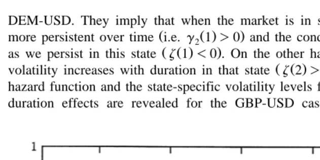
DEM-USD. They imply that when the market is in state 1, this state becomes

Ž Ž . .

more persistent over time i.e.g2 1 )0 and the conditional volatility decreases

Ž Ž . .

as we persist in this state z 1 -0 . On the other hand, in state 2, conditional

Ž Ž . .

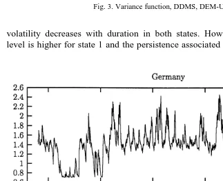
volatility increases with duration in that state z 2 )0 . Figs. 2 and 3 plot the hazard function and the state-specific volatility levels for the DEM-USD. Similar duration effects are revealed for the GBP-USD case, except that conditional

(15)

Fig. 3. Variance function, DDMS, DEM-USD.

volatility decreases with duration in both states. However, the initial volatility level is higher for state 1 and the persistence associated with that state is stronger.

(16)

Unconditional probabilities for S from the DDMS model can be computed ast

Ž . Ž . Ž .

P S sÝdP S, Dsd , where P S, D , Ss1,2, 1FDFt are the joint

uncondi-Ž .

tional probabilities associated with S and D . P S for the DEM-USD are 0.39t t ŽSts1 and 0.61 S. Ž ts2 , and those for the GBP-USD are 0.80 S. Ž ts1 and 0.20. ŽS_ts2 ..

Ž .

Ljung-Box test statistics for autocorrelation 10 and 20 lags in the squared standardized residuals appear at the bottom of the table. According to this diagnostic, all of the models appear to capture serial correlation in the squared standardized residuals. This suggests that using duration as an instrument in the conditional variance and transition matrix is a substitute for ARCH.

Fig. 4 plots the estimates of volatility for the DDMS specification. To calculate the conditional standard deviations implied by the DDMS model, we use Eq.

Ž3.22 along with the parameter estimates reported in Table 2. Note that the.

DDMS model is able to capture abrupt discrete changes in volatility.

5. Adequacy of the conditional distributions

To properly manage short-term risk, the conditional distribution of returns must be correctly specified. The maintained statistical model will influence a risk assessment, such as VaR, primarily through the time-varying dynamics of condi-tional volatility.14 _{As discussed in Section 1, a risk manager will not only be}

concerned with whether or not VaR assessments are correct on average, but also with the adequacy of such predictions at each point in time.

This section evaluates the models’ conditional distributions. We begin by assessing out-of-sample interval forecasts associated with a particular coverage level. We then use a density forecast test which has more statistical power for tail areas of the distribution since the test exploits the level of the realization as well as the indicator of whether or not it falls in the desired interval. This increased statistical power is particularly useful for relatively short data samples for which realizations in the tail may be few in number. Finally, we report results for the

Ž .

density test DT using the entire distribution and the full sample of available data.

5.1. InterÕal forecasts

Traditionally, the most common approach to assessing a time-series volatility model has been to compare the out-of-sample forecast to some proxy of latent volatility. Volatility is sometimes measured by squared forecast errors or squared returns. For a correctly specified model, this measure of volatility is consistent but noisy. The result is that conventional tests have low power to reject constant

14

(17)

volatility models in favour of time-varying ones. As Andersen and Bollerslev

Ž1998 show, the noise associated with using squared returns to measure latent.

volatility can be substantial.

An alternative approach is to consider out-of-sample interval forecasts. This is attractive because no latent measure of volatility is needed. In addition, interval forecasts depend not only on the volatility dynamics but also on the conditional mean specification and the conditional density. Thus, analysis of a models’ interval forecasts provide information about the suitability of the maintained conditional distribution of returns.

Ž .

We follow the testing methodology of Christoffersen 1998 and test for correct conditional coverage associated with out-of-sample interval forecasts. Tests associ-ated with conditional coverage involve a joint test of coverage plus independence. That is, correct unconditional coverage only assesses the total number of realiza-tions in the desired interval. It does not preclude the possibility of temporal dependence in the realization of hits in or out of the desired interval. Clustering of a particular realization would indicate neglected dependence in the conditional volatility model, or more generally, in the maintained conditional distribution. The joint test is derived in a maximum likelihood framework using the appropriate

Ž .

likelihood ratio LR as a test statistic. First, define

L

Ž .

p ,U

Ž .

p

Ž

5.1

.

Ž

tNty1 tNty1

.

as the ahead interval with desired coverage probability p. This one-step-ahead interval forecast, for a particular model and information set Vty1, is computed as

where F 1ypr2 is the inverse cumulative distribution function of the

Ž .

normal distribution evaluated at 1ypr2. That is, we focus on symmetric interval forecasts.15

A model with correct coverage, given information at ty1, has the property that the realized y falls in the desired interval with probability p. That is,t

P L

Ž

tNty1

Ž .

p -yt-UtNty1

Ž .

p NVty1

.

sp.

Ž

5.4

.

15

Using the normal distribution for critical values would be consistent with the modeling assumption for a GARCH model but should be considered an approximation for the forecasted density associated with an MS model. More computationally oriented interval forecast methods, including the bootstrap,

Ž .

(18)

The parameters of the models discussed in Section 3 are estimated with the information set VNy1, Ny1-T, and thereafter assumed fixed, while the data

from N to T is used to evaluate the out-of-sample forecasts. We set Ny1s1000, leaving 304 observations for out-of-sample interval tests.16

4T

for tsN, . . . ,T. This indicator variable records, for each t, whether or not the

Ž .

forecast interval Eq. 5.1 contained the realized value y ._t

Now, consider a test for correct conditional coverage, which is defined as,

w

x

E ItNIty1, Ity2, . . . sp

Ž

5.6

.

Ž .

for all t. Christoffersen 1998 shows that correct conditional coverage implies

4 Ž .

that It ;IID Bernoulli p under the null hypothesis. This test can be

decom-posed into two individual tests. The first is a test for correct unconditional

w x w x

coverage E It sp, vs. the alternative E It /p, while the second test is for

4

independence of the binary sequence I , . . . , I .N T

The likelihood under the null hypothesis of correct conditional coverage is

n0 _n

1

in which n and n are the number of zeroes and ones, respectively, from the data₀ ₁

I , . . . , I . Following Christoffersen 1998 , we consider a first-order Markov_N _T4 Ž .

chain alternative for which the likelihood is

P; I , . . . , IN T

_.

Ž

5.9

.

2_{Ž .}

which will be distributed x 2 under the null hypothesis. Note that the restric-tions implied by that null hypothesis of correct conditional coverage arep₁₁sp

Ž .

andp₀₀s 1yp .

16

(19)

Table 3 reports, for each model and currency, p-values associated with the joint

Ž .

test for correct conditional coverage labeled IF for a desired symmetric coverage level of 0.8. That is, we are evaluating an interval forecast, which covers the middle 80% of the distribution. Recall that this test associated with conditional coverage is a joint test of correct unconditional coverage and independence.

Ž . Ž

Although this test rejects a linear AR 1 model with constant variance p-values

.

are 0.02 and 0.00 for the DEM-USD and GBP-USD, respectively , it is unable to reject either of the time-varying volatility parameterizations for the DEM case. On the other hand, all models are rejected for the GBP-USD application. Our results indicate that the rejection of correct conditional coverage for this currency is due

Ž .

to failure to capture average unconditional coverage rather than due to violation of independence.

For a well-specified model, we would expect the interval-forecast tests to pass for a wide range of desired coverage levels. In other words, we want forecasts of the model to be accurate for different regions of the distribution. Although conceptually, we could compute the p-values associated with a wide range of desired coverage levels, statistical power will depend on how many realizations fall outside and inside the chosen interval. As the interval approaches the whole distribution, the outside region will disappear so that the test cannot be imple-mented. On the other hand, choosing a desired coverage corresponding to, for example, the lower tail of the distribution, may result in a relatively small number of realizations inside the interval. In either case, the test will lack statistical power to discriminate between the null and the alternative and consequently between the models. For these cases, an alternative strategy to evaluating the conditional density is required.

Table 3

Distribution test results

Test Germany UK

MS-ARCH DDMS MS-ARCH DDMS

Out-of-Sample Forecasts

IF 0.209 0.137 0.0005 0.0011

DT-full 0.012 0.030 0.1e-5 0.0065

In-Sample Forecasts

DT-tail 0.075 0.348 0.011 0.029

Ž .

The interval forecast IF test is a joint LR test for correct coverage and independence based on

Ž . Ž .

Christoffersen 1998 with a desired coverage level of 0.8. The density tests DT are LR tests

ŽBerkowitz, 1999 for the adequacy of the maintained models distribution — DT-full for the entire.

(20)

5.2. Density forecasts

A closely related family of tests on a models distributional assumptions is

Ž . Ž .

detailed in Diebold et al. 1998 and Berkowitz 1999 . The tests are based on the

Ž . Ž .

integral transformation of Rosenblatt 1952 . Suppose that f ytNVty1 is the conditional distribution of y based on the information sett Vty1. Then Rosenblatt

Ž1952 shows that.

y_t

u_ts

H

f

Ž

ÕNV_t_y₁

.

dÕ, tsN, . . . ,T ,

Ž

5.10

.

y`

Ž .

is IID and uniformly distributed on 0,1 . Therefore, a researcher can construct

T

_˜

Diebold et al. 1998 suggest graphical methods in order to assess how f P

Ž .

fails in approximating the true unknown density, while Berkowitz 1999 suggests

4T

applying the inverse normal transformation to u

˜

t tsN in order to test whether or

4T

not the transformed series z_{t t}_s_N is independent standard normal. An attractive feature of the latter approach is that we can use any of the exact tests based on

17 _Ž _.

normality. In particular, following Berkowitz 1999 , we consider LR tests for several applications. By construction, these tests involve a continuous variable and

Ž .

not a discrete indicator variable as in the interval forecast tests Section 5.1 . For this reason, and also due to the use of LR statistics, we expect these tests to have good power properties in finite samples.18

y1_{Ž .} y1_{Ž .}

First, define ztsF u , where

˜

t F P is the inverse of the standard normal distribution function. Then, under the null hypothesis of the correct density,

Ž .

zt;NID 0,1 . The first LR test is based on the following regression,

ztsmqr

Ž

zty1ym

.

qw .t

Ž

5.11

.

Ž .

The null hypothesis is msrs0,Var wt s1 whereas, the alternative is

Ž . 19

m/0, r/0, Var wt /1. This test may identify problems in the unconditional distribution and also time dependences not captured by the conditional dynamics.

Ž .

The first panel of Table 3 reports p-values for this LR test labeled DT-full associated with density forecasts using the same out-of-sample period tsN, . . . ,T

used for the interval forecasts reported in Section 5.1. The relevant integrals were computed numerically, utilizing quadrature. Broadly speaking, this test produces

17

The LR test is exact only in the case of hypothesis tests in which z follows a normal distributiont

under both the null and alternative.

18_{Traditional tests on u}₄T _{for IID behaviour generally will not have good power. However,}

˜t tsN

Ž .

Berkowitz 1999 shows that applying the inverse normal transformation to u , and using classical˜t

tests, results in good power properties in finite samples.

19

It should be noted that these tests do not take into account sampling variability in estimating the

˜Ž .

(21)

conclusions similar to the interval-forecast tests with respect to the alternative currencies. However, the p-values are lower, so that there are marginal rejections for the DEM-USD as well. The DDMS model is not as strongly rejected as the MS-ARCH, however, both models appear to be missing important features in the data. Note however, that we did not update parameter estimates after each one-step ahead forecast. Doing so might result in a more favourable result for the postulated distributions.

Ž

Finally, we also compute a LR test that focuses on lower-tail behaviour as in

.

VaR which can be constructed based on a truncated normal distribution. The loglikelihood for the truncated normal zt-a is

2

Since the number of realizations in the tail will be small, we computed this DT

Ž .20

using the entire sample ts1, . . . ,T . The in-sample results for the lower tail

Žas y1.645 are reported in Table 3, in row DT-tail. Again, these results favour.

Ž . Ž .

the DDMS parameterization. As a further comparison the AR 1 -GARCH 1,1

Ž . Ž .

model had a p-value of 0.006 DEM-USD and 0.004 GBP-USD for the DT-tail test. These results for the left tail of the distribution concord well with our measures of the unconditional distribution discussed in the next section which show that the duration-dependent parameterization captures excess kurtosis more adequately.

Our results suggest that volatility is forecastable at a weekly frequency and that a constant volatility model for exchange rates can be a poor choice. Moreover,

Ž .

unlike the tests conducted by West and Cho 1995 , these interval and density forecast tests show the value of richer models in tracking conditional volatility. We have found that the DDMS parameterization outperforms the GARCH and MS-ARCH model, but is still strongly rejected by the UK weekly data.

6. Features of the unconditional distributions

Earlier sections showed that the addition of high-order dependence through duration dependence in the DDMS model allows for rich conditional density

20

(22)

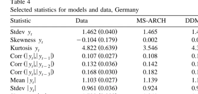
Table 4

Selected statistics for models and data, Germany

Ž .

Statistic Data MS-ARCH DDMS GARCH 1,1

Ž .

Stdev yt 1.462 0.040 1.465 1.469 1.619

Ž .

Skewness yt y0.104 0.179 0.002 0.002 0.010

Ž .

Kurtosis yt 4.822 0.639 3.546 4.340 6.091

Ž< < < <. Ž .

Mean yt 1.103 0.027 1.139 1.116 1.220

< < Ž .

Stdev yt 0.961 0.036 0.924 0.958 1.065

< < Ž .

Skewness yt 1.722 0.233 1.249 1.584 2.106

< < Ž .

Kurtosis yt 8.401 1.756 4.904 6.715 13.297

< < Ž .

Mean log yt y0.379 0.033 y0.314 y0.353 y0.256

< < Ž .

Stdev log yt 1.174 0.031 1.144 1.157 1.147

< < Ž .

Skewness log yt y1.157 0.089 y1.414 y1.346 y1.363

< < Ž .

Kurtosis log yt 4.738 0.382 6.510 6.308 6.369

Data is 100 times the log first-difference in the exchange rate. For each model, one draw of sample size 1 000 000 was used to calculate the sample statistic. Standard errors robust to heteroskedasticity appear in parenthesis. The parameter values in Table 2 are assumed to be the true model parameters.

dynamics for foreign currency rates. This section shows that the DDMS parameter-ization also provides a more flexible structure when matching unconditional moments.

Monte Carlo methods are used to compute some summary measures of the unconditional distributions implied by the alternative volatility parameterizations. To estimate the simulated moments, we draw a sample of size 1 000 000 from the conditional distribution implied by the maintained model, and calculate a battery of summary statistics.21 _{These simulated moments can then be compared to the}

Ž .

corresponding moments and standard errors estimated from the actual data. Tables 4 and 5 report these numbers for the DEM-USD and GBP-USD cases, respectively.

The simulated statistics for the MS models match those observed in the data more closely than those from the plain vanilla GARCH model, and in some cases, those for the DDMS model match better than the MS-ARCH model. Consider, for example, the results for the DEM-USD case. The standard deviation from the DDMS and MS-ARCH models is much closer to that found in the data than is the GARCH estimate. In addition, the GARCH model produces too much kurtosis,22 the MS-ARCH produces too little kurtosis, while the estimate for the DDMS

21

The first 20 000 draws were dropped to eliminate dependence on startup conditions.

22

(23)

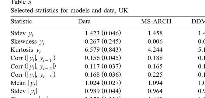
Table 5

Selected statistics for models and data, UK

Ž .

Statistic Data MS-ARCH DDMS GARCH 1,1

Ž .

Stdev yt 1.423 0.046 1.458 1.432 1.411

Ž .

Skewness yt 0.267 0.245 0.006 0.012 0.011

Ž .

Kurtosis yt 6.579 0.843 4.244 5.163 3.691

Ž< < < <. Ž .

Mean yt 1.024 0.027 1.094 1.049 1.102

< < Ž .

Stdev yt 0.989 0.044 0.964 0.975 0.882

< < Ž .

Skewness yt 2.258 0.234 1.463 1.844 1.339

< < Ž .

Kurtosis yt 11.376 1.940 6.189 7.815 5.736

< < Ž .

Mean log yt y0.500 0.034 y0.427 y0.476 y0.330

< < Ž .

Stdev log yt 1.216 0.034 1.241 1.245 1.124

< < Ž .

Skewness log yt y1.131 0.103 y1.294 y1.347 y1.453

< < Ž .

Kurtosis log yt 5.009 0.454 5.749 6.158 6.709

See notes in Table 4.

parameterization is within one standard error of that for the data. For the GBP-USD case, the standard deviation of y is matched by all models, but in thist case, both the GARCH and MS-ARCH models produce too little kurtosis while the DDMS parameterization is within two standard errors of the kurtosis estimate for the data.

The DDMS model also fits better than a simple first-order MS model. For example, the unconditional standard deviation and kurtosis measures associated with a first-order MS model are 1.46 and 3.54 for the DEM-USD.23_{As shown in}

Ž .

Table 4, the kurtosis associated with the data is 4.822 standard error, 0.639 and that implied by the DDMS model is 4.340. In the GBP-USD case, the first-order MS model yields an unconditional kurtosis measure of 4.43 while the data has

Ž .

6.579 standard error, 0.843 and DDMS has 5.163. These results, as well as other simulation results for the simpler MS models, point to the duration dependence structure in the DDMS model providing a closer fit to the unconditional distribu-tion of the weekly changes in foreign exchange rates.

< < < <

Many of the summary measures for y and log y , which we can interpret ast t alternative proxies for volatility, are also captured better by the DDMS parameteri-zation. For example, for the DDMS parameterization applied to the DEM-USD, all

< <

of the first four moments of volatility as measured by y are within one standardt error of the data estimate, whereas none of them are for either the MS-ARCH or

Ž < <.

GARCH models. For volatility clustering measured by the autocorrelation in y ,t

23

Ž .

These were computed using parameter estimates available on request for a first-order MS model

Ž .

(24)

Fig. 5. y Models vs. data, Germany.t

there is not much to choose from between the alternative parameterizations. However, the MS-ARCH model does slightly better for the DEM-USD case whereas DDMS and GARCH are marginally better for the GBP-USD currency.

To complement the results reported in Tables 4 and 5, Figs. 5 and 6 present kernel density plots of the data and of the simulated unconditional distributions for

< <

y and log y implied by the DDMS and GARCH models. 1 000 000 draws weret t taken from the respective models. These data were used to estimate the density, assuming a Gaussian kernel and a constant bandwidth that is optimal for the normal distribution with the variance calculated from the data. The plots were robust to a wide range of bandwidth parameters.

<

(25)

The figures support the conclusion that the DDMS parameterization provides a good description of the unconditional distributions. For instance, Fig. 5 shows that DDMS captures the density of y for the DEM-USD quite well around the origin, while GARCH does not. This is consistent with the GARCH model putting too

Ž .

much mass in the tail and resulting in a higher kurtosis than in the data Table 4 .

Ž . < <

Similarly, for the GBP-USD Fig. 6 , the distribution of log y is closer to the_t data for the DDMS parameterization, although neither model captures this log absolute value transformation very well. This evidence is consistent with that presented in earlier sections of the paper, that is, although the DDMS model is preferred, none of the parameterizations fully capture the structure in the GBP-USD case.

7. Concluding comments

The last section showed that the DDMS could account for many of the properties of the unconditional distribution of y and functions of y usuallyt t associated with measures of volatility. Unlike GARCH parameterizations, the DDMS structure allows time-varying persistence, includes a stochastic component for volatility, and incorporates anticipated discrete changes in the level of volatil-ity. The DDMS model is an example of a mixture of distributions model. As reviewed in Section 1, MS models are well-known to have the ability to produce various shaped distributions including skewness and leptokurtosis. Our plots of unconditional distributions for DDMS confirm those results.

According to our results, including the out-of-sample interval and density forecast tests reported in Section 5, the DDMS parameterization is also a good statistical characterization of the conditional distribution of foreign exchange

Ž

returns. This is in contrast to earlier studies for example, Pagan and Schwert,

.

1990 which have shown that simpler MS models cannot capture all of the volatility dependence.

(26)

The empirical distribution generated by our proposed structure is a superior match for the samples of data used in this paper. These enhancements may be particularly relevant for forecasts necessary for risk management. However, it is still difficult to fully capture the distributions of log-differences of the GBP-USD

Ž .

exchange rate see Gallant et al., 1991 . More work remains to be done.

8. Model summary

Ž .

GARCH 1,1

ysmqfy qe, s2_s_v_q_ae2 _q_bs2 _,

t ty1 t t ty1 ty1

etsstz ,t zt;N 0,1 .

Ž

.

Ž .

MS-ARCH p

y_tsmqfy_t_y₁qe_t

etss

Ž .

St z ,t zt;N 0,1 ,

Ž

etss

Ž .

St z ,t zt;N 0,1 ,

Ž

P S

Ž

.

s . 1qexp

Ž

g1

Ž .

2 qg2

Ž .

2 dty1

.

Acknowledgements

(27)

Institute of Financial Economics and Journal of Empirical Finance Conference on Risk Management held at Albufeira, Portugal, November 1999; participants at the Canadian Econometrics Study Group held at the University of Montreal, Septem-ber, 1999; and Clifford Ball, Adolf Buse, Peter Christoffersen, Toby Daglish, Jin-Chuan Duan, Ronald Huisman, Chang-Jin Kim, Pok-sang Lam, Simon van Norden, and Ilias Tsiakas for helpful comments and discussions. We also thank Werner Antweiler for providing data. Both authors thank the Social Sciences and Humanities Research Council of Canada for financial support.

References

Andersen, T.G., Bollerslev, T., 1998. Answering the skeptics: yes, standard volatility models do

Ž .

provide accurate forecasts. International Economic Review 39 4 , 885–905. Berkowitz, J., 1999. Evaluating the Forecasts of Risk Models. Federal Reserve Board.

Bollerslev, T., 1986. Generalized autoregressive conditional heteroskedasticity. Journal of Economet-rics 31, 309–328.

Boothe, P., Glassman, D., 1987. The statistical distribution of exchange rates. Journal of International Economics 22, 297–319.

Cai, J., 1994. A Markov model of switching-regime ARCH. Journal of Business & Economic Statistics

Ž .

12 3 , 309–316.

Chatfield, C., 1993. Calculating interval forecasts. Journal of Business & Economic Statistics 11, 121–135.

Ž .

Christoffersen, P.F., 1998. Evaluating interval forecasts. International Economic Review 39 4 , 841–862.

Diebold, F.X., 1988. Empirical Modeling of Exchange Rate Dynamics. Springer, Berlin.

Diebold, F.X., Gunther, T.A., Tay, A.S., 1998. Evaluating density forecasts with application to

Ž .

financial risk management. International Economic Review 39 4 , 863–883.

Durland, J.M., McCurdy, T.H., 1994. Duration-dependent transitions in a Markov model of U.S. GNP

Ž .

growth. Journal of Business & Economic Statistics 12 3 , 279–288.

Engle, C., Hamilton, J.D., 1990. Long swings in the dollar: are they in the data and do markets know it? American Economic Review 80, 689–713.

Engle, R.F., 1982. Autoregressive conditional heteroskedasticity with estimates of the UK inflation. Econometrica 50, 987–1008.

Evans, M.D.D., 1996. Peso problems: their theoretical and empirical implications, Handbook of Statistics vol. 14 Elsevier, Chap. 21.

Filardo, A.J., 1994. Business cycle phases and their transitional dynamics. Journal of Business &

Ž .

Economic Statistics 12 3 , 299–308.

Gallant, A.R., Hsieh, D.A., Tauchen, G.E., 1991. Nonparametric and semiparametric methods in econometrics and statistics and econometrics. On Fitting a Recalcitrant Series: The PoundrDollar Exchange Rate, 1974–1983. Cambridge Univ. Press, pp. 199–240.

Ghysels, E., Harvey, A.C., Renault, E., 1996. Stochastic volatility, Handbook of Statistics vol. 14 Elsevier, Chap. 5.

Gray, S.F., 1996. Modeling the conditional distribution of interest rates as a regime-switching process. Journal of Financial Economics 42, 27–62.

(28)

Hamilton, J.D., 1989. A new approach to the economic analysis of non-stationary time series and the business cycle. Econometrica 57, 357–384.

Hamilton, J.D., 1994. Time Series Analysis. Princeton Univ. Press, Princeton, NJ.

Hamilton, J.D., Susmel, R., 1994. Autoregressive conditional heteroskedasticity and changes in regime. Journal of Econometrics 64, 307–333.

Hsieh, D., 1989. Testing for nonlinearity in daily foreign exchange rate changes. Journal of Business 62, 339–368.

Kaehler, J. and Marnet, V., 1993,AMarkov-Switching Models for Exchange-Rate Dynamics and the Pricing of Foreign-Currency Options,BZEW Discussion paper No. 93-03.

Kim, C.J., Nelson, C.R., 1998. Business cycle turning points, a new coincident index, and tests of duration dependence based on a dynamic factor model with regime switching. Review of

Eco-Ž .

nomics and Statistics 80 2 , 188–201.

Kim, C.J., Nelson, C.R., Startz, R., 1998. Testing for mean reversion in heteroskedastic data based on

Ž .

Gibbs-sampling-augmented randomization. Journal of Empirical Finance 5 2 , 131–154. Klaassen, F., 1998. Improving GARCH Volatility Forecasts. Tilburg University.

Lam, P., 1997, AA Markov switching model of GNP growth with duration dependence,B Federal Reserve Bank of Minneapolis, Discussion Paper 124.

Lindgren, G., 1978. Markov regime models for mixed distributions and switching regressions. Scandinavian Journal of Statistics 5, 81–91.

Maheu, J.M., McCurdy, T.H., 2000. Identifying bull and bear markets in stock returns. Journal of

Ž .

Business & Economic Statistics 18 1 , 100–112.

Nieuwland, F., Vershchoor, W., Wolff, C., 1994. Stochastic trends and jumps in EMS exchange rates. Journal of International Money and Finance 13, 699–727.

Pagan, A., 1996. The econometrics of financial markets. Journal of Empirical Finance 3, 15–102. Pagan, A., Schwert, G.W., 1990. Alternative models for conditional stock volatility. Journal of

Ž .

Econometrics 45 1–2 , 267–290.

Palm, F.C., 1996. GARCH models of volatility, Handbook of Statistics vol. 14 Elsevier, Chap. 7. Perez-Quiros, G., Timmermann, A., 1999. Firm size and the cyclical variations in stock returns. Journal

of Finance, in press, in Journal of Finance.

Rosenblatt, M., 1952. Remarks on a multivariate transformation. Annals of Mathematical Statistics 23, 470–472.

Ryden, T., Terasvirta, T., Asbrink, S., 1998. Stylized facts of daily returns series and the hidden´ ¨

Markov model. Journal of Applied Econometrics 13, 217–244.

Taylor, S.J., 1999,AMarkov processes and the distribution of volatility: A comparison of discrete and continuous specifications,BLancaster University, Management School, working paper 99r001. Timmermann, A., 2000. Moments of Markov switching models. Journal of Econometrics 96, 75–111. Vlaar, P.J.G., Palm, F.C., 1993. The message in weekly exchange rates in the european monetary system: mean reversion, conditional heteroscedasticity, and jumps. Journal of Business & Economic

Ž .

Statistics 11 3 , 351–360.