www.elsevier.nlrlocaterjappgeo
Improvement in TDEM sounding interpretation in presence of
induced polarization. A case study in resistive rocks of the Fogo
volcano, Cape Verde Islands
Marc Descloitres
a,), Roger Guerin
b, Yves Albouy
a, Alain Tabbagh
b, Michel Ritz
a´
a
IRD, Laboratoire de Geophysique, 32 a´ Õenue H. Varagnat, 93143 Bondy Cedex, France
b
Departement de Geophysique Appliquee, UMR 7619 Sisyphe, Uni´ ´ ´ Õersite Pierre et Marie Curie, case courrier 105,´ 4 place Jussieu, 75252 Paris Cedex 05, France
Received 24 June 1999; accepted 4 May 2000
Abstract
Ž .
A Time Domain Electromagnetic TDEM survey was carried out in and around the caldera of the Fogo volcano, Cape Verde Islands, to detect the low resistive structures that could be related to groundwater. A sign reversal in the sounding curves was encountered in central-loop measurements for the soundings located in the centre of the caldera along three main radial profiles. The negative transients are recorded in the early channels between 6.8 and 37ms. Negative values in an early time transient is an unusual field observation, and consequently the first step was to check the data to ascertain their
Ž .
accuracy and quality. In the second step, three-dimensional 3D effects are evaluated and ruled out in this zone, while an
Ž . Ž .
Induced Polarization IP phenomenon is observed using Direct Current DC sounding measurements. In the third step, the IP effect is called upon to explain the TDEM distortions; a Cole–Cole dispersive conductivity is found to be adequate to fit
Ž .
the field data. However, the more relevant one-dimensional 1D model is recovered when both central-loop and offset-loop data are jointly taken into account, thus indicating that an effect of dispersive conductivity is necessary to explain the field data. The 1D electrical structure exhibits four layers, with decreasing resistivity with depth. Only the first layer is polarizable and its Cole–Cole parameters are ms0.85, cs0.8 and ts0.02 ms for chargeability, frequency dependence and time constant, respectively. However, the Cole–Cole parameters deduced from TDEM forward modelling remain different from those deduced from DCrIP sounding. In this volcanic setting, this IP effect may be caused by the presence of small grains
Ž .
of magnetite andror by the granularity of effusive products lapillis . As a conclusion, it is shown that a modelling using different TDEM data sets is essential to recover the electrical structure of this area.q2000 Elsevier Science B.V. All rights reserved.
Keywords: Central-loop TDEM; Negative transient; Induced Polarization; Cole–Cole modelling; Fogo volcano
)Corresponding author. IRD, Geophysique BP 182, Ouagadougou, Burkina Faso. Tel.:q226-30-67-37; fax:q
226-31-03-85.
Ž . Ž . Ž
E-mail addresses: [email protected] M. Descloitres , [email protected] Y. Albouy , [email protected] A.
. Ž .
Tabbagh , [email protected] M. Ritz .
0926-9851r00r$ - see front matterq2000 Elsevier Science B.V. All rights reserved.
Ž .
1. Introduction
During the last 20 years, Induced Polarization
ŽIP effects in Time Domain Electromagnetism.
ŽTDEM have been reported in field surveys..
Resulting distortions of the sounding curves cannot be explain by common 1D models, and may lead to erroneous interpretation if the IP effect is not recognised. Among the papers deal-ing with IP effects, many describe the theoreti-cal and field data obtained using coincident-loop or central-coincident-loop configurations. The more severely distorted TDEM curves show negative data at the end of the transients, which are not expected in such geometrical configurations.
Many authors have modelled distorted ground response by frequency-dependent conductivities
ŽSpies, 1980; Lee, 1981; Walker and Kawasaki, 1988; Flis et al., 1989; Kaufman et al., 1989; Smith and West, 1989; Elliott, 1991;
El-.
Kaliouby et al., 1995; El-Kaliouby et al., 1997 . The Cole–Cole formula introduces three polar-ization parameters: the Cole–Cole chargeability
Ž .m , the frequency dependence Ž .c , and the
Ž .
Cole–Cole time constant t . All studies agree
that the Cole–Cole model is adequate to take into account the IP effect observed in TDEM. These procedures are generally motivated by the
Ž .
necessity to i recover the true resistivity model
Ž
of the ground see, e.g. Flis, 1987 or Hohmann
.
and Newman, 1990 for 3D polarizable bodies ,
Ž .ii enhance the IP response in order to better
Ž
characterise IP target parameters El-Kaliouby
. Ž .
et al., 1995, 1997 , iii estimate IP parameters
Ž
of clays in hydrogeological surveys Everett,
.
1997 . Theoretical papers have also investigated the possible separation between IP and induc-tive responses. For this purpose, Kamenetsky
Ž .
and Timofeyev 1984 suggested deploying dif-ferent sizes of transmitter loop in order to pro-vide different data sets used for the modelling.
Ž .
Kaufman et al. 1989 explore the influence of Cole–Cole parameters for three common trans-mitter–receiver configurations — central-loop, coincident-loop and dipole–dipole. Under cer-tain conditions, they separate the inductive and
polarizable parts of the response. Another
prac-Ž .
tical approach is proposed by McNeill 1994 who advocates the use of offset-loop soundings in order to attenuate or even avoid the IP distor-tions obtained in central-loop configuration.
Fi-Ž .
nally, Kamenetsky and Novikov 1997 propose a physical modelling approach in order to get laboratory measurements on rock samples.
When dealing with the interpretation of dis-torted TDEM curves using a dispersive model, the interpreter is confronted with many equiva-lent models. In addition to resistivity and thick-ness, three unknown Cole–Cole parameters are needed to fit the field data. Some rules have been pointed out when investigating the influ-ence of Cole–Cole parameters upon TDEM
Ž
curves Kaufman et al., 1989; El-Kaliouby et
.
al., 1997 . Even so, the interpretation is still difficult and does not necessarily lead to an unique model. Consequently, the determination of the resistivities and thicknesses could remain uncertain.
This study was primarily motivated by the need to interpret central-loop data with sign reversal that are obtained when prospecting for aquifers inside the caldera of the Fogo volcano,
Ž .
Cape Verde Islands Descloitres et al., 1995 . For this survey, the distorted transients are un-usual because the negatives occur at the begin-ning of early time portion of the curves. This is contrary to most of the studies previously men-tioned, where the negatives occur at the end of
Ž
the curves, or in the middle of the curves
«dou-.
ble sign reversal» as Walker and Kawasaki
Ž1988 or Barsukov and Fainberg 1998 no-. Ž .
offset-loop data obtained at the same site into the modelling procedure. This allows us to
demon-Ž .
strate that i the IP effect is effectively re-moved or attenuated when larger transmitter loop or offset-loop configurations are used and
Ž .ii multi-data modelling improves the interpre-tation allowing a better determination of the Cole–Cole parameters as well as the geoelectri-cal model.
2. Survey setting
The data presented here are a part of a TDEM survey for groundwater carried out inside the caldera of the Fogo volcano. The 25-km-diame-ter island is an active hot spot of the Cape Verde Islands. This archipelago, 600 km from the coast of west Africa, is semi-desert. The rainfall on Fogo varies between 200 and 1000
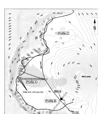
Fig. 1. Topographic map of the caldera and main peak of the Fogo volcano. The location of the TDEM sites are indicated
Ž . Ž .
with blank squares 1994 survey . Filled square: test site B4 presented in this study 1995 survey . Area in gray: location of the 1995 lava flows. The dashed line separates TDEM points into two zones: the TDEM curves from points situated between
Ž
this line and the caldera rim do not show any negative values and detect shallow conductive layers not presented in this
.
mm a year in locations related to prevailing winds. The inhabitants are facing with many problems due to insufficient water supply. Rain-water penetrates into the highly permeable sur-face materials, a phenomenon that leads to cru-cial irrigation problems. The caldera is a large semi-cylindrical structure 1750 m high bordered
Ž
to the west by a 500- to 1000-m high wall Fig.
.
1 . This caldera has a diameter of 8 km and the bottom is a flat terrain considered as the main
Ž
recharge zone for groundwater Barmen et al.,
.
1990 . The caldera is filled by volcanic prod-ucts. The surface generally consists in dry pa-hoehoe and lava flows, lapillis andror ashes. Geophysics has been considered here in order to detect conductive layers that could be related to groundwater. Previous tests of the
audiomagne-Ž .
totelluric AMT method were done. They were unsuccessful principally because of poor AMT signal, strong topographic effects and many dif-ficulties in getting good ground contacts for telluric measurements. TDEM measurements were carried out at the same time, and were found to be more effective.
3. Method and data acquisition
The TDEM method is a controlled source
Ž .
electromagnetic EM method that uses a large loop laid on the ground as a transmitter. A current is alternatively turned on and off in the loop. When the current is flowing, a primary static EM field is created. When the current is turned off, an EMF produces eddy currents flowing in the earth, diffusing further into the formation. The eddy currents create a secondary EM field whose amplitude decreases with time. During the absence of current in the transmitter, this EM field due to eddy current in the earth is measured on the surface by a receiver coil. The shape of the decay voltage, or transient, with time depends on the ground resistivity distribu-tion and the array configuradistribu-tion. The transmitter loop can be laid out using various configura-tions, depending on the objectives of the survey.
The most common for shallow applications are the central-loop, coincident-loop and offset-loop modes. For a comprehensive review of the TDEM method, see Nabighian and MacNae
Ž1991 or McNeill 1994 .. Ž .
A Geonics PROTEM 47 system was chosen in our first survey in 1994, because it was easy to handle over difficult terrains. We laid out a 100=100 m2 transmitter loop for central-loop measurements. A total of 117 soundings sites were covered within 17 days. They are located along three main radial profiles and the contours
Ž .
of the caldera Fig. 1 . The distorted TDEM curves are mainly located along the three pro-files. A second survey dedicated to the study of the distorted transient was carried out in 1995. Both EM 47 and 37 systems were deployed on the test site B4 located in the south of the
Ž .
caldera Fig. 1 , which was the only accessible place after the eruption of the volcano in April 95.
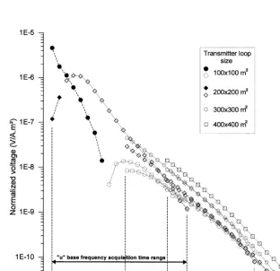
The PROTEM system allows TDEM data to be acquired using several base frequencies. Each frequency-based acquisition typically result in 20 normalized voltages logarithmically spaced in time. For EM 47, two overlapping base fre-quencies were recorded — «u» 237.5 Hz and « v» 62.5 Hz, with time sampling from 6.8ms to 2.79 ms. The EM 37 system has a higher trans-mitter voltage, and two overlapping base fre-quencies were recorded — «H» 25 Hz and
«M» 6.25 Hz, with time sampling from 88 ms
to 27.8 ms. For the last channels of the «M» base frequency and the large transmitter mo-ments, measurements show that the noise level is reached. The following measurements were made on site B4:
Ø central-loop measurements using four differ-ent square transmitter loops: 100=100, 200
=200, 300=300 and 400=400 m2;
Ø offset-loop measurements using 100=100
m2 transmitter loop and 100, 150 and 200 m
offsets;
Ø measurements of the primary field along a
measurements of three component of the time-varying secondary magnetic field have been performed in order to evaluate if any 2D or 3D structures occur beneath this site.
In order to complete our study of site B4, Direct
Ž .
Current DC and time domain IP Schlumberger soundings were carried out using a SYSCAL-R2 resistivity-meter from IRIS Instruments.
4. Field data at site B4
4.1. Central loop TDEM data
The data for site B4 are presented in Fig. 2 as normalized voltage vs. time for overlapping «u»,
«H» and «M» base frequencies. The « v» base frequency is omitted here to simplify the figure. For 100=100 m2 data recorded at «u» base
frequency, the first eight channels show
nega-tive data from 6.8 to 37 ms; the other 12
channels remain positive. For the 200=200 m2
data, only the first two channels are negative. For all of the curves recorded at «H» and «M» base frequencies, as well as for 300=300
and 400=400 m2 transmitters, there are no
negative data.
It should be noted that negative responses occur in the early part of the decay, before 37
ms, and would not have been observed with any
TDEM equipment starting acquisition 37 ms
after the turn-off time. Furthermore, the nega-tive part of the signal is less important or
ishes when larger transmitter loop or offset-loop configurations are used.
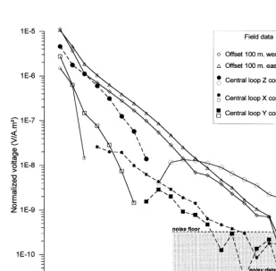
4.2. Offset-loop and 3D TDEM data
Offset-loop measurements were acquired at the four cardinal points from the cable, at off-sets of 100, 150 and 200 m. Fig. 3 presents the 100 m offset curves west and east of the 100=
100 m2 loop transmitter. Those curves are close
together and always positive.
For the 3D measurements, the X and Y com-ponents measured at the centre show that tran-sient levels remain one decade below the Z component level and fall into EM and
instru-mental noise between 100 and 300 ms.
According to offset-loop measurements, there is no evidence of 3D structure beneath this site that would explain central-loop TDEM distor-tions.
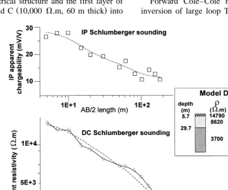
4.3. DC and IP Schlumberger soundings
Both DC and IP Schlumberger soundings
Ž .
reveal i a decreasing apparent resistivity curve
from 15,000 to 5000 V m for an ABr2 length
Ž .
of 200 m and ii a decreasing IP apparent
chargeability curve from around 30 to 10
mVrV. The weighted average of the apparent
chargeability is calculated with the four regis-tered time windows, ranging from 160 to 1580 ms after the current turn-off. The evidence of a
Fig. 3. TDEM offset-loop and 3D central-loop field data measured at site B4 at «u» base frequency. The filled symbols and dashed lines indicate negative values, blank symbols and continuous lines are positive values. North and south offset-loop data as well as 150 and 200 m offset data are omitted here for clarity, and remain identical to the west and east transient. The
time domain electrical IP response in such ground is an indication to consider an IP effect to explain the distortions of TDEM curves in an earlier range of time.
5. Quality control of the data
As already noted, the occurrence of negative data in the first part of a central-loop transient has never been reported in published papers. Therefore, it is logical to suspect any problem linked to acquisition process that could pro-duced such distortions. Below, we evaluate pos-sible field errors or instrumental problems: the inversion of the polarity, a non-synchronous acquisition or inappropriate receiver bandwidth, and a transmitter, i.e. turn-off effect.
5.1. Control of the polarity of the data
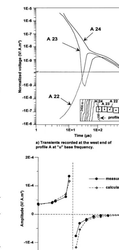
The data acquired in 1994 at the three adja-cent sites A22, A23 and A24 at the west end of
Ž .
profile A Fig. 1 are presented in Fig. 4a. At these sites, the duration of the negative part of the transient reduces itself when the loop is moved closer to the rim. At site A24, the curve remains entirely positive. This shows a progres-sive attenuation or even the disappearance of the phenomenon and ascertains that the sign of the responses are correct, i.e. that the negatives are present in the first part of the transient.
To reinforce this assertion, Fig. 4b shows the shape of the primary field recorded at several locations of the receiver moving across the 100
=100 m2 transmitter loop at site B4. The
theoretical primary field is also calculated for this loop. It remains close to the field data. According to Lenz law for central-loop acquisi-tion, the sign of the primary field is identical to the sign of the secondary field when the mea-surements are made after a current turn-off. In our case, the primary field remains positive in the centre of the loop while the first measured windows exhibit negative values. This fact leads
Ž .
Fig. 4. a Example of three sounding curves obtained at the west end of profile A with 100=100 m2 central-loop
Ž .
array configuration. b Comparison between the primary field measured at site B4 and the primary field calculated for a 100=100 m2 transmitter loop for different locations
of the receiver coil crossing the loop.
5.2. Non-synchronous acquisition or inappro-priate receiÕer bandwidth
Improper timing of the acquisition could lead to the fact that the first windows of the transient should have been registered during the turn-off of the primary signal. In the same way, a limited receiver bandwidth could integrate the receiver response to the primary field so it extends into the time window of early measure-ments. As told above, for a central-loop acquisi-tion, the primary and secondary fields should have the same polarity after a current turn-off. Therefore, any synchronisation problem locat-ing the acquisition time into the turn-off time should only manifest itself by an increasing
amplitude of early time positive measurements, but never in reversing their polarity. In the case of limited receiver bandwidth, the effect is to delay the response, but never to reverse the sign
ŽGeonics, pers. comm. . This fact is confirmed.
Ž .
by Effersø et al. 1999 .
5.3. Transmitter turn-off effect
In high resistive ground conditions, the re-sponse of the transmitter loop to an abrupt
Ž 2 .
turn-off time 5.2 ms in a 100=100 m loop
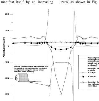
could lead to an improper shape of the current ramp, which exhibits some oscillations around zero, as shown in Fig. 5. If such a condition
Ž .
Fig. 5. Comparison between the shapes and the signs of: i the secondary field measured at site B4 for two time windows of
Ž . Ž .
11.8 and 18 ms, ii the secondary field calculated for a half-space of 10,000 V m, and iii the residual primary field resulting from a hypothetical improper turn-off time for different receiver locations crossing the 100=100 m2 transmitter
exists, a residual primary field with opposite polarity could be present at the end of the ramp leading to the following remark: if a negative response observed in the central-loop is due to residual negative current flowing into the trans-mitter loop in reaction to an improper turn-off, there should exists a strict amplitude relation between this signal and the signal observed at the different offset locations. This residual sig-nal in offset should indeed have the same varia-tion in time, an inverse polarity, i.e. positive if the signal at the centre is negative, and a de-creasing amplitude when the offset distance in-creases.
For further illustration, we have drawn in Fig. 5 the amplitude of the transient vs. the receiver location for the time windows at 11.8 and 18 ms. Inside the transmitter loop, where the residual primary field is supposed to be negative, the sign of the secondary field is also negative, but their shapes are not the same. Outside the transmitter loop, the signs remain identical, but again their shapes are not the same; the amplitude of the primary field de-creases abruptly with increasing distance, while the secondary field is increasing at the same time to reach an amplitude relatively constant in accordance with normal behaviour, as shown as an example for the calculated response over a
half-space of 10,000 V m.
These results indicate that the negative sec-ondary field in the centre of the loop cannot be related to any residual negative current flowing into the transmitter loop.
6. Data modelling
The occurrence of an IP signal in conven-tional DCrIP sounding, as well as the progres-sive disappearance of negative transients when larger transmitter loop central-loop or offset-loop configurations are used, leads us to attempt forward modelling of the data with Cole–Cole dispersive conductivity.
6.1. Some aspects of TDEM 1D modelling using Cole–Cole parameters
The influence of IP effects on TDEM curves is mostly discussed for the coincident-loop
con-Ž
figuration Kaufman et al., 1989; El-Kaliouby et
.
al., 1997 and sometimes for the central-loop
ŽElliott, 1991 or offset-loop soundings Everett,. Ž .
1997 . These publications use the Cole–Cole
Ž
model Cole and Cole, 1941; Pelton et al.,
.
1978 . The formulation expresses the ground
Ž
conductivity as a dispersive
frequency-depen-.
dent conductivitys:
c
Cole–Cole chargeability 0FmF1 , c the
fre-Ž .
quency dependence 0FcF1 , t the Cole–
Ž .
Cole time constant s , and v the angular
fre-Ž .
quency Hz .
Among many results provided by the afore-mentioned papers, the following conclusions were obtained for coincident-loop and central-loop configurations in time domain.
ØThe part of the TDEM response due to the
IP effect is negative. In some situations, when the amplitude of the inductive part of the re-sponse becomes small enough, the IP signal dominates and leads to negative data. This oc-curs usually at late time.
ØThe more resistive the ground, the higher the amplitude of the IP effect. In general, it can be shown that the amplitude of negative peaks is roughly proportional to the square root of the resistivity.
ØWhen sign reversal are recorded, the time of occurrence and amplitude of the negative peak are strictly connected with the value of m,
c and t.
Ž .
described by Kaufman et al. 1989 for
central-Ž .
loop systems. El-Kaliouby et al. 1997 deter-mine an optimum loop radius to enhance the amplitude of the phenomenon for coincident-loop system over a polarizable half space. This leads to a better determination of the Cole–Cole parameters of the target.
For a defined polarizable model, these studies point out that the transmitter–receiver configu-ration governs the shape and the amplitude of the IP effect.
6.2. Forward modelling of the TDEM data us-ing Cole–Cole parameters
The 1D code we used for magnetic TDEM
Ž
response forward modelling Tabbagh and
.
Dabas, 1996 was modified to take into account a Cole–Cole conductivity behaviour. For each layer, the conductivity can be complex and is described by the Cole–Cole formula. The cur-rent turn-on and turn-off times are described by considering a series of successive step functions to follow the Geonics current waveform. The calculation of the transient response is provided either at the centre of the transmitter loop or at any offset location, and is given for the Geon-ics-defined time windows.
The Cole–Cole forward modelling of the 100
=100, 200=200 m2 central-loop and 100 m
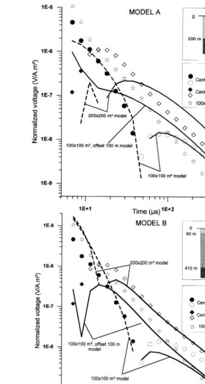
offset-loop data at «u» base frequency is pre-sented in Fig. 6. First, we tried to fit the 100=
100 m2 central-loop data: a preliminary model,
A, consists in a two-layer structure with the first layer having a resistivity r of 10,000 V m and 200 m thick and its Cole–Cole parameters are
ms0.65, cs0.5 and ts0.l ms. The second
layer is conductive of rs250 V m and
non-polarizable. The model fits the 100=100 m2
central-loop data with a good agreement. The voltage response for the model A is then calcu-lated for 200=200 m2and 100 m offset data. It is quite different from the field data. Hence, the model A cannot be considered as relevant, be-cause it fits only the 100=100 m2 central-loop
data. Therefore, we decided to take into account
Fig. 6. Cole–Cole forward modelling of «u» base fre-quency transients for 100=100, 200=200 m2central-loop
and 100 m offset field data. The filled symbols and dashed lines indicate negative values, blank symbols and continu-ous lines are positive values. The lines are the resulting calculated transients for model A and B.
larger loop sizes and offset-loop data to improve the model.
Ž .
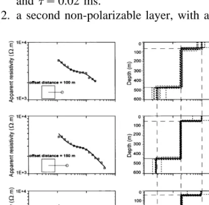
illustrated in Fig. 7 for «u» base frequency acquisition. For the three sets of offset-loop data, the models are almost identical and equiv-alence analysis determines an average three-layer model showing:
1. a resistive, 3000–70 000 V m, first layer of 35–90 m thick;
2. an intermediate resistive, 1700–2200 V m,
second layer of 370–420 m thick;
3. a low resistive, 190–600 V m, basement.
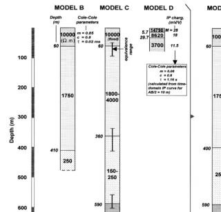
In a third step, this three-layer solution was taken as a starting solution for a forward mod-elling of the central-loop data including Cole– Cole parameters. After some trial and error, the model B shows:
1. a resistive, polarizable first layer of 60 m
thick, with resistivity of 10,000 V m and
Cole–Cole parameters of ms0.85, cs0.8
and ts0.02 ms.
2. a second non-polarizable layer, with a
resis-Fig. 7. 1D inversion of the data acquired at site B4 with «u» base frequencies for offset distances of 100, 150 and 200 m from the centre of the 100=100 m2 transmitter loop. The inversion is made using TEMIX software. The averaged model deduced from these inversions is used as a starting solution in Cole–Cole forward modelling resulting
Ž .
in model B see text .
tivity of approximately 1750 V m and thick-ness of about 350 m; and
3. a non-polarizable conductive layer of 250 V
m resistivity.
In Fig. 6, the resulting curves for 100=l00,
200=200 m2 central-loop and 100 m
offset-loop configuration are presented. For the 100= 100 m2central-loop configuration, model B does not fit the field data as well as model A did, but the amplitude of the negative part and time of sign reversal fits the data reasonably well. For the 200=200 m2 central-loop and offset-loop
configurations, the resulting curves of model B fit the field data reasonably well. Attempts have been made to improve the fit of the last part of the 100=100 m2 field data and to evaluate the
equivalence ranges of the Cole–Cole parame-ters. If their values are changed more than 5–10%, the resulting synthetic transients do not fit any of the three TDEM field data sets. This confirms that the use of different data sets im-proves the definition of the model as was al-ready pointed out by Krivochieva and Chouteau
Ž1997 for a non-dispersive medium. It is found.
to be the case also in dispersive medium. At this stage, model B appears to be more relevant than model A, even if its fit remains imperfect to the late part of the 100=100 m2
central-loop data. The following observations are to be noted.
ØThe Cole–Cole modelling allows the
re-covery of a transient shape close to the field data, including negatives in the first part of the transients, provided that high values of charge-ability and frequency dependence, as well as short time constant, are chosen. This does not necessarily proves that an IP effect is the only possible explanation for the sign reversal, but shows that an IP effect cannot be ruled out to explain the sign reversal phenomenon.
ØModel A shows a conductive layer of 250
V m at a depth of 200 m. The more relevant
model B shows a conductive layer of 250 V m
used to model the data, a severe misinterpreta-tion can occur.
ØThe resistivities and thicknesses deduced from non-dispersive 1D inversion offset-loop data remain close to those calculated with
Ž .
Cole–Cole forward modelling model B . This tends to confirm that offset-loop data are less affected by any IP effect.
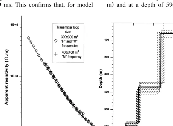
6.3. Interpretation of 300=300 and 400=400 m2 central-loop low base frequency data
In order to validate the presence and the depth of the conductive layer in this part of the caldera, we have conducted a 1D inversion
us-ing 300=300 and 400=400 m2 central-loop
data at «H» and «M» base frequencies.
A forward calculation of the dispersive model B was computed for both configurations. The results show that the presence of the first polar-izable layer does not significantly modify the transient response for time windows between 88
ms and 2.79 ms. This confirms that, for model
B with late transient and larger transmitter loop, the inductive part of the response is much more predominant than the polarizable part of the response originated by the first layer.
These results allow us to conduct a 1D inver-sion, presented in Fig. 8 as apparent resistivity vs. time for «H» and «M» base frequencies. Using model B as a starting solution for upper layers, but without any Cole–Cole parameters, a fourth layer has been added in order to fit the data and results in model C as follows:
Ž . Ž .
Layer Resistivity range V m Thickness m
Ž .
1 10,000 fixed 60
2 1800–4000 300
3 150–250 230
4 50 –
Model C confirms the presence of a conduc-tive layer of 150–250 V m at a depth of 360 m, which is close to the model B solution of 250 V
m and 410 m deep. Moreover, this inversion
Ž
defines a fourth layer more conductive 50 V
.
m and at a depth of 590 m, which could not
logically be determined by higher base fre-quency transients.
6.4. Modelling of DCrIP sounding data
In order to detail the uppermost part of the geoelectrical section where model B describes a resistive polarizable layer of 60 m thick, we have carried out a joint inversion of DC and IP sounding data using the software of Sandberg
Ž1993 . The results are presented in Fig. 9. The.
resulting model D consists of a three-layer structure as follows:
Layer Resistivity Thickness chargeability
ŽV m. Ž .m ŽmVrV.
1 14,790 5.7 28
2 8620 24 18
3 3700 – 11.5
This joint inversion details the upper part of the geoelectrical structure and the first layer of
Ž .
model B and C 10,000 V.m, 60 m thick into
three resistive layers. The values of IP charge-ability are decreasing regularly with depth. An attempt have been made to transform the raw
Ž .
chargeability data mVrV for the four time
windows obtained for ABr2 length of 10 m
into Cole–Cole parameters using a software developed by IRIS Instrument for the SYSCAL
Ž .
R2 data. For a fixed frequency dependence c
Ž .
of 0.8, the chargeability m and the time
con-Ž .
stant t are 0.06 and 1.16 s, respectively.
Those results have to be taken with caution because the raw data are measured over only four time windows with this equipment, which gives a poor sampling of the IP transient decay. Even with this precaution, those values are far
from ms0.85 and ts0.02 ms deduced from
TDEM forward modelling in model B.
6.5. Final model
Ž .
Forward Cole–Cole modelling model B ,
Ž .
inversion of large loop TDEM data model C
Ž .
Fig. 10. Comparison between models B, C, D and E. Model B is from Cole–Cole forward modelling of 100=100, 200=200 m2 central-loop and offset-loop TDEM data with «u» base frequency. Model C is from 1D inversion of
300=300 and 400=400 m2central-loop TDEM data with «H» and «M» base frequencies. Model D is from joint inversion
of DC and IP Schlumberger soundings. Model E is an average model derived from models B and C, which can be proposed as the resistivity structure below site B4 — results from model D only detail the shallower part of the first resistive layer and are omitted in model E.
Ž .
and joint inversion of DCrIP data model D
are presented in Fig. 10. An average model, E, can be derived taking into account the informa-tion given by these models. The first layer has a
resistivity of 10,000 V m, is 60 m thick, and
remains the only polarizable layer. Its Cole– Cole parameters deduced from TDEM Cole–
Cole forward modelling are ms0.85, cs08
andts0.02 ms. The interpretation of’ the DC sounding divided it into three layers with
resis-tivity and thicknesses of 14,790 V m, 5.7 m
thick, 8620 V m, 24 m thick and 3700 V m;
and IP chargeability of 28, 18 and 11.5 mVrV, respectively of depth. The second layer is less
Ž .
resistive 1750 V m and 340 m thick. The
Ž .
third layer is conductive 250 V m and 190 m
Ž
thick. The ultimate layer is conductive 50 V
.
m and is only revealed by large transmitter loop TDEM data.
7. Discussion
The first point to be discussed is our ap-proach to model TDEM data using a dispersive conductivity. Once the quality of the data has been ascertained, three main considerations are
Ž .
Cole–Cole formula as reported in the literature;
Ž .ii the accordance of the raw TDEM data set to theoretical studies, which mention the attenua-tion of the IP effect when larger transmitter loop
Ž .
or offset-loop configuration are used; and iii the occurrence of IP signal measured in conven-tional DCrIP sounding. The forward modelling has shown that model B describes the distorted transients, and moreover satisfies the predicted behaviour when multi-data sets are taken into account. Thus, we believe that dispersive con-ductivity is a possible explanation for our dis-torted transients. However, parametrization of conventional IP chargeability data obtained with the Schlumberger sounding into the Cole–Cole formulation fails to reconcile the values of m
and t with their corresponding values deduced
from TDEM forward modelling. At this stage of the study, we believe that this discrepancy can-not be explained in a simple manner with such data set. But this is not surprising due to the difference in time constants between conven-tional IP and TDEM, which leads us to the second point of our discussion related to the origin of the IP effect in a volcanic setting.
According to the work on spectral IP by
Ž .
Pelton et al. 1978 , it is possible to encounter
Ž .
high chargeabilities m )0. 8 and short time
Ž .
constant t -0.1 ms with rocks containing
more than 20% of sulfides and a grain size less than 0.l mm. Moreover, one sample of mag-netite from Iron Mount, UT, USA, exhibits a chargeability near l.0 and a time constant near 0.08 ms. Another example of high chargeability
Ž0.5 and short time constant 0.69 ms has been. Ž .
calculated from distorted central-loop TDEM measurements for resistive permafrost formation
Ž .
of 1000 V m by Walker and Kawasaki 1988 .
In our case, the origin of the IP effect has to involve dry lapillis and massive lava flows for-mation. To the best of our knowledge, such an IP effect involving TDEM has not been reported yet for volcanic areas. Some TDEM studies over volcanoes have already been carried out
ŽJackson and Keller, 1972; Jackson et al., 1986;
.
Fitterman et al., 1988 . These studies did not
take note of negative voltage in TDEM data, but the transients were recorded at times of a few tens of milliseconds, much later than ours.
Ž .
Patella et al. 1991 describe examples of
fre-Ž .
quency dispersion in magnetotellurics MT data in deep geothermal volcanic zones. The IP ef-fect is attributed to hydrothermal paragenesis, which cannot be taken into account in our shal-lower case. As clearly described by Flis et al.
Ž1989 , the IP effect is generally caused by.
metallic mineral grains andror negatively
charged clay disseminated in the rock. In our case, we have to rule out the implication of shallow clay layers, which would have been detected in DC sounding as conductive layers. However, the anomalous TDEM soundings are located in our study over thicknesses of tens of meters of lapillis. This material can contain
Ž .
small particles of magnetite -0.1 mm and
produce an IP effect in the high frequency range. This fact has to be investigated further to be able to confirm this behaviour, and the pres-ence of small particles does not explain the
longer time constant of ts1.16 s calculated
from DCrIP sounding in the lower frequency
range. We believed that an IP effect with a longer time constant could be generated by the granularity of the lapillis having grains of more than 1-mm diameter. This raises the question that if two IP effects with two time constants could coexist why have they not been detected
by both TDEM or DCrIP soundings? To
an-swer this question, two calculations have been done. The first one is the TDEM response for the dispersive model B, with Cole–Cole param-eters of the first layer fixed to the values of
ms0.06, cs0.8 andts1.16 s, deduced from
DCrIP sounding. The TDEM response does not
differ from a non-dispersive case, that indicates that 100=100 m2 central-loop high base
mod-Ž .
elling model B . For the four time windows,
the IP response remains near 0.01 mVrV,
be-Ž
low the practical measurable amplitude Iris
.
Instruments, pers. comm. . Those calculations show that if two IP effects could coexist the shorter one is only revealed by the EM 47
equipment and the longer one by the DCrIP
SYSCAL R2 instrument.
It should be noted here that normal transients, i.e. positive values, have been recorded in other places of the volcano, where lapillis could also be present, and consequently the exact origin of the IP effect cannot be ascertain with our data set alone and would require laboratory work on rock samples.
The third point of our discussion refers to other possible causes of distorted transients
Ž . Ž .
linked with i displacement currents and ii magnetic viscosity.
Displacement currents are usually neglected in conventional modelling. But when an imagi-nary part is considered for s, a corresponding permittivity ´ is implicitly considered and the
true permittivity effect remains negligible
against the imaginary part of the conductivity effect: the results of the forward modelling us-ing dispersive model B and a dielectric constant of 3 for the first layer does not show any
difference compared with the ´s0 case for
transients measured 6.8 ms after the current
turn-off time.
Magnetic viscosity effects in TDEM data are largely documented in archaeological
prospec-Ž
tion Colani and Aitken, 1966a; Mullins and
.
Tite, 1973; Dabas and Skinner, 1993 and also
Ž
in mining prospection Buselli, 1982; Spies and
.
Frischknecht, 1991 . This phenomenon leads to late time distortion, but never reverses the sign of central-loop or coincident-loop data. We be-lieve that this phenomenon can be ruled out to explain our sign reversal.
The last point to be discussed here is the geological implications of the average model E. As no drilling information is available in this area, we should note that the general resistivity structure is noticed in other studies. Fitterman et
Ž .
al. 1988 has encountered resistive first layers over deep conductive zones in the Newberry volcano. On the flanks of Piton de la Fournaise
Ž .
volcano Reunion Island , moderately deep
300–500 m conductive layers have been de-tected and attributed to aquifers and clayey
Ž .
formations Descloitres et al., 1997 . For the averaged model E derived in this study, the resistive first and second layers are attributed to recent dry volcanic formations of basaltic lava, lapillis or ashes. The third intermediate-resistiv-ity layer is attributed to partially or totally wa-ter-saturated volcanic rocks alone or those asso-ciated with clayey layers between fractured lava flows. The conductive basal layer is attributed to the old volcanic complex-clayey zone related to deep alteration of the volcanic rocks andror hydrothermal zone.
8. Conclusions
Recording negative data with the TDEM cen-tral-loop configuration should lead to suspect an
Ž .
IP dispersive conductivity effect. Therefore, to be able to quantify and model the TDEM re-sponse, we acquired data using several transmit-ter loop sizes as well as different positions of the receiver coil.
For shallow applications in case of highly resistive polarizable superficial formations, par-ticularly in such volcanic setting, central-loop measurements using small transmitter loops, i.e.
F100=100 m2, should be avoided. The
off-set-loop data as well as larger loop size mea-surements are less affected by IP effects. A Cole–Cole model compared to only one set of data can lead to severe misinterpretation. Con-sequently, in order to be able to get a more relevant model, one should acquire several field data set of different loop sizes andror offset locations and incorporate them into the mod-elling. In our case a relevant dispersive model
Ž .
Ž .
and ii Cole–Cole modelling through trial and error of central-loop and offset-loop data using various transmitter loop sizes. This procedure greatly improves the determination of resistiv-ity, thickness and Cole–Cole parameters.
Regarding our survey, TDEM method was found to be an adequate way of prospecting low resistivity zones in such volcanic settings but the IP effect detected in some places can be troublesome when attempting to recover the geoelectrical section. The origin of the IP effect detected in this area remains difficult to deter-mine, but the modelling shows that this effect is related to a shallow resistive layer. Using differ-ent data sets, the global electrical structure of the central part of this caldera can be estimated. Cole–Cole forward TDEM modelling remains difficult to practice. Any inversion model of different data sets which takes into account Cole–Cole parameters, should help to recover more relevant solutions. No doubt that in other favorable conditions, AMT soundings or large DC soundings could be jointly interpreted with TDEM data in order to give a more constrained image of the subsurface.
Acknowledgements
This work took place as a part of the
Ž
GEAQUIF research Program of IRD Institut de
.
Recherche pour le Developpement . The 1995
´
field campaign was partially supported by the
Ž
Cap-Verdian Institute INGRH Instituto
Na-.
cional de Gestao dos Recursos Hidricos and the
ˆ
Mission de Cooperation Franc
´
¸
aise in Praia. We wish to thank the two reviewers as well as N.B. Christensen for their constructive criticisms, M. Chouteau from Ecole Polytechnique de Montreal´
for providing the EM-37 equipment, H. El-Kaliouby for earlier discussions and suggestions to improve the TDEM Cole–Cole models, M. Goldman and M. Bosnar for fruitful discussions on TDEM IP distortions and P.Valla from IRIS Instruments for his help on the conversion of
DCrIP data into Cole–Cole parameters. We are grateful to A. Querido, J. Descloitres and N. Mademba for their field contributions.
References
Barmen, G., Carvalho, V. and Querido, A., 1990. Ground-water-related geological and isotopic investigations on the Island of Fogo. An overview. Lund University and INIT file report, Praia, 72 pp.
Barsukov, P.O., Fainberg, E.B., 1998. Double IP Effect in electromagnetic transients. 14th Workshop on Electro-magnetic Induction in the Earth, Sinaia, August 16–22. pp. 97–98, Abstracts, paper 6.4.
Buselli, G., 1982. The effect of near-surface superparam-agnetic material on electromsuperparam-agnetic measurements.
Ž .
Geophysics 47 9 , 1315–1324.
Colani, C., Aitken, M.J., 1966a. Utilisation of magnetic viscosity in soils for archaeological prospection. Nature 212, 1446–1447.
Cole, K.S., Cole, R.H., 1941. Dispersion and absorption in dielectrics. 1 — Alternating current. J. Chem. Phys. 9, 341–351.
Dabas, M., Skinner, J., 1993. Time domain magnetisation
Ž .
of soils VRM , experimental relationship to quadrature
Ž .
susceptibilities. Geophysics 58 3 , 326–333.
Descloitres, M., Ritz, M., Mourgues, P., 1995. TDEM soundings for locating aquifers inside the caldera of the Fogo active volcano, Cape Verde Islands. Proceedings of the 1st Meeting of EEGS European Section, Sept 25–27, Torino. pp. 110–114.
Descloitres, M., Ritz, M., Robineau, B., Courteaud, M., 1997. Electrical structure beneath the eastern collapsed flank of Piton de la Fournaise volcano, Reunion Island: implication to the quest for groundwater. Water Resour.
Ž .
Res. 33 1 , 13–19.
Effersø, F., Auken, E., Sørensen, K.I., 1999. Inversion of band limited TEM responses. Geophys. Prospect. 47, 551–564.
El-Kaliouby, H.M., Hussain, S.A., Bayoumi, A., El-Di-wany, E.A., Hashish, E.A., 1995. Effect of clayey media parameters on the negative response of a
coinci-Ž .
dent loop. Geophys. Prospect. 43 5 , 595–603. El-Kaliouby, H.M., El-Diwany, E.A, Hussain, S.A.,
Hashish, E.A., Bayoumi, A.R., 1997. Optimum nega-tive response of a coincident-loop electromagnetic
sys-Ž .
tem above a polarizable half-space. Geophysics 62 1 , 75–79.
Elliott, P., 1991. An empirical procedure for removal of polarisation effects observed in TEM field data. Explor.
Ž .
Everett, M.E., 1997. Transient inductive coupling of loops over near-surface clay-bearing sandstones. 67th Ann.
Ž .
Internat. Mtg. Dallas, TX, November 2–7 , Soc. Expl. Geophys.
Fittermann, D.V., Stanley, W.D., Bisdorf, R.J., 1988. Elec-trical structure of Newberry volcano, Oregon. J.
Geo-Ž .
phys. Res. 93 B9 , 10119–10134.
Flis, M., 1987. IP effects in 3D TEM data— theory and
Ž .
case histories. Explor. Geophys. 18 1 , 55–58. Flis, M.F., Newman, G.A., Hohmann, G.W., 1989.
In-duced-polarization effects in time-domain
electromag-Ž .
netic measurements. Geophysics 54 4 , 514–523. Hohmann, G.W., Newman, G.A., 1990. Transient
electro-magnetic response of superficial, polarizable patches
Žshort note . Geophysics 55 8 , 1098–1100.. Ž .
Jackson, D.B., Keller, G.V., 1972. An electromagnetic sounding survey of the summit of Kilauea volcano,
Ž .
Hawaii. J. Geophys. Res. 77 26 , 4957–4965. Jackson, D.B., Frischknecht, F.C., Kauahikaua, J., 1986.
Three-layer inversions for 18 TDEM soundings in the cone crater area, SW rift zone of Kilauea volcano, Hawaii. U.S. Geol. Surv. Open-file Rep. 87-76. Kamenetsky, F.M., Timofeyev, V.M., 1984. Possibility to
separate induction and polarization transients. Phys.
Ž .
Earth 12, 89–94, in Russian .
Kamenetsky, F.M., Novikov, P.V., 1997. A physical study of low-frequency dispersion of rock conductivity in time-domain electromagnetics. Geophys. Prospect. 45
Ž .3 , 421–434.
Kaufman, A.A., Geoltrain, S., Knoshaug, R.N., 1989. In-fluence of induced polarization in inductive methods. Geoexploration 26, 75–93.
Krivochieva, S., Chouteau, M., 1997. Improvement in TDEM interpretations by joint inversion of different
Ž .
data sets. 3rd Mtg. Aarhus, September 8–11 , Euro-pean Section of Environmental and Engineering Geo-phys. Soc., Proceedings. pp. 347–350.
Lee, T., 1981. Transient electromagnetic response of a
Ž .
polarizable ground. Geophysics 46 7 , 1037–1041. McNeill, D.J., 1994. Principles and applications of time
domain electromagnetic techniques for resistivity soundings. Geonics, technical note TN 27.
Mullins, C.E., Tite, M.S., 1973. The magnetic properties of soils and their application to archaeological prospect-ing. Archaeophysika 5, 143–347.
Nabighian, M.N., Macnae, J.C., 1991. Time domain elec-tromagnetic prospecting methods. In: Nabighian, M.N.
ŽEd. , Electromagnetic Methods in Applied Geo-.
physics. Applications vol. 2 SEG publication, pp. 427– 520, Chap. 6.
Patella, D., Tramacere, A., Di Maio, R., Siniscalchi, A., 1991. Experimental evidence of resistivity frequency-dispersion in magnetotellurics in the Newberry
ŽOregon , Snake River Plain Idaho and Campi Flegrei. Ž . ŽItaly. volcano-geothermal areas. J. Volcanol. Geotherm. Res. 48, 61–75.
Pelton, W.H., Ward, S.H., Hallof, P.G., Sill, W.R., Nel-son, P.H., 1978. Mineral discrimination and removal of inductive coupling with multifrequency IP. Geophysics
Ž .
43 3 , 588–609.
Sandberg, S.K., 1993. Examples of resolution improve-ment in geoelectrical soundings applied to groundwater
Ž .
investigations. Geophys. Prospect. 41 2 , 207–227. Smith, R.S., West, G.F., 1989. Field examples of negative
coincident-loop transient electromagnetic responses modeled with polarizable half-planes. Geophysics 54
Ž11 , 1491–1498..
Spies, B.R., 1980. A field occurrence of sign reversal with the transient electromagnetic method. Geophys.
Ž .
Prospect. 28 4 , 620–632.
Spies, B.R., Frischknecht, F.C., 1991. Electromagnetic
Ž .
Sounding. In: Nabighian, M. Ed. , Electromagnetic Methods in Applied Geophysics. Applications vol. 2 SEG publications, Chap. 5.
Tabbagh, A., Dabas, M., 1996. Absolute magnetic viscos-ity determination using time-domain electromagnetic devices. Archaeol. Prospection 4, 199–208.