Directory UMM :Data Elmu:jurnal:J-a:Journal of Econometrics:Vol101.Issue1.2001:

(1)

Robust inference with GMM estimators

Elvezio Ronchetti

!

, Fabio Trojani

",

*

!Department of Econometrics, University of Geneva, Blv. Carl Vogt 102, CH-1211 Geneva, Switzerland "Institute of Finance, University of Southern Switzerland, Via G. Buz13, 6900 Lugano, Switzerland

Received 1 September 1999; received in revised form 1 April 2000; accepted 5 July 2000

Abstract

The local robustness properties of generalized method of moments (GMM) estimators and of a broad class of GMM based tests are investigated in a uni"ed framework. GMM statistics are shown to have bounded in#uence if and only if the function de"ning the orthogonality restrictions imposed on the underlying model is bounded. Since in many applications this function is unbounded, it is useful to have procedures that modify the starting orthogonality conditions in order to obtain a robust version of a GMM estimator or test. We show how this can be obtained when a reference model for the data distribution can be assumed. We develop a#exible algorithm for construct-ing a robust GMM (RGMM) estimator leadconstruct-ing to stable GMM test statistics. The amount of robustness can be controlled by an appropriate tuning constant. We relate by an explicit formula the choice of this constant to the maximal admissible bias on the level or (and) the power of a GMM test and the amount of contamination that one can reasonably assume given some information on the data. Finally, we illustrate the RGMM methodology with some simulations of an application to RGMM testing for conditional heteroscedasticity in a simple linear autoregressive model. In this example we

"nd a signi"cant instability of the size and the power of a classical GMM testing procedure under a non-normal conditional error distribution. On the other side, the RGMM testing procedures can control the size and the power of the test under non-standard conditions while maintaining a satisfactory power under an approxi-matively normal conditional error distribution. ( 2001 Elsevier Science S.A. All rights reserved.

*Corresponding author. Tel.:#41-91-912-4723.

E-mail addresses:elvezio.ronchetti@metri.unige.ch (E. Ronchetti), fabio.trojani@lu.unisi.ch (F. Trojani).

(2)

MSC: C12; C13; C14

Keywords: ARCH models; GMM estimators and tests; In#uence function; Robust model selection; Robustness of validity

1. Introduction

This paper analyzes the local robustness properties of estimators based on the GMM (cf. Hansen, 1982) and of test statistics based on a GMM estimator. We characterize the local robustness of GMM estimators, of Hansen's speci"cation test and of GMM-based tests that are GMM versions of the classical Wald, score, and likelihood-ratio test (cf. Newey and West, 1987a; Gourieroux and Monfort, 1989) by a single property: the boundedness of the underlying ortho-gonality function. Since many available econometric models are based on an unbounded orthogonality function, we propose a simple uni"ed setting for constructing a robust GMM (RGMM) estimator yielding at once the local robustness of all GMM-based tests.

The need for robust statistical procedures for estimation, testing and predic-tion has been stressed by many authors both in the statistical and econometric literature; cf. for instance, Hampel (1974), Koenker and Bassett (1978), Huber (1981), Koenker (1982), Hampel et al. (1986), Peracchi (1990, 1991), Markatou and Ronchetti (1997), Krishnakumar and Ronchetti (1997). This paper focuses on locally robust GMM estimation and testing and contributes to the current literature in the following directions.

First of all, our results extend the application of robust instrumental variables estimators proposed by Krasker and Welsch (1985), Krasker (1986) and Lucas et al. (1994) to a general GMM setting with nonlinear orthogonality conditions and where some stationary ergodic dependence in the underlying data generat-ing process is admitted.

Secondly, the paper generalizes the robust testing framework developed by Heritier and Ronchetti (1994) to a general GMM setting. It uni"es and simpli"es the theory by proposing a RGMM estimator leading to robust Wald, score and likelihood-ratio type tests for general nonlinear parameter restrictions.

Finally, the paper provides some robust versions of Hansen's speci"cation test. This yields RGMM model selection procedures that were not available before.

(3)

nonparametric GMM situation. However, in many applications of the GMM, the reference model distribution is already implied by the problem under investigation (for instance in the case of normality of the error distribution). Furthermore, when no natural reference model is supplied we claim that it is often useful to impose one in order to obtain GMM statistics that behave su$ciently well at least over a restricted set of relevant model distributions. The implied orthogonality conditions are then approximate in the sense that they should be satis"ed by any model distribution&near' }in some appropriate sense

}to the given reference model. When translating this argument in terms of the empirical distribution of the data, this means that in a RGMM framework a small fraction of the observations can deviate from the rest of the sample without a!ecting the empirical moment conditions in a dramatic way. There-fore, the derived parameter estimates and statistics are representative for the structure of the&majority'of the data. In other words, robust GMM procedures pay a small&insurance premium'in terms of e$ciency at the reference model in order to be robust in a neighborhood of it.

At least in linear models with normal serially independent errors, the e!ects of di!erent kinds of distributional deviations from the assumptions are well studied and known to have an important impact on the asymptotic properties of a GMM estimator; cf. Krasker and Welsch (1985), Krasker (1986) and Lucas et al. (1994). For the time-series context important work has been done by KuKnsch (1984) and Martin and Yohai (1986) within the framework of (linear) autoregressive models. Since there is a priori no reason to generally believe that in a nonlinear model with stochastic time dependence these e!ects should be less serious, a general RGMM framework can o!er a powerful complement to the classical GMM in many applications.

In this paper we focus on locally robust GMM estimation and particularly on GMM testing, that is on smooth GMM functionals that can be locally approximated by means of their in#uence function (IF); see Hampel (1968, 1974) and Hampel et al. (1986) for basic de"nitions and KuKnsch (1984) and Martin and Yohai (1986) for the time-series context. Boundedness of the IF implies that in a neighborhood of the model the bias of an estimator cannot become arbitrarily large. In the testing framework this implies that in a neighborhood of the model the level of the test does not become arbitrarily close to 1 (robustness of validity) and the power does not become arbitrarily close to 0 (robustness of e$ciency). Hence, a bounded in#uence function is a desiderable local stability property of a statistic.

Since in applications the IF of a GMM statistical functional is often un-bounded (some examples are listed in Section 2), we propose a robusti"ed version of a GMM estimator that is shown to induce at the same time (locally) robust GMM testing procedures. The RGMM estimator is constructed by applying a basic truncation argument of the theory of robust statistics

(4)

proposed estimator is that the amount of robustness imposed can be controlled by a tuning constant which is related by an explicit formula to both the maximal local bias in the level and the power of a GMM test and to the magnitude of the given model deviation; see Section 4.

As an illustration of these general principles consider for instance a simple AR(1) model with ARCH(1) (cf. Engle, 1982) errors for a random sequence (y

t)t|N: y

t"b0#b1yt~1#Jhtut, ht"a0#a1u2t~1, (1)

where (u

t)t|N is a standardized i.i.d. sequence with unknown distribution. A natural set of orthogonality conditions for a GMM estimation of the parameters (a₀, a₁, b₀,b₁) is given by

E[e_t]"0, E[e_ty

t~1]"0, E[gt!ht]"0, E[gtgt~1]"0, (2)

where

e_t"y

t!b0!b1yt~1, gt"e2t. (3)

We will see that the unboundedness of the orthogonality function de"ning these orthogonality conditions implies a lack of robustness of GMM estimators and tests. For this case we propose a small simulated application to testing for a conditional heteroscedasticity speci"cation in the linear autoregressive model. In this simple experiment we observe that for relevant sample sizes the classical GMM procedure is unstable even under relatively small distributional devi-ations from the normality of the error distribution. Speci"cally, the GMM speci"cation test often produces sizes that are higher than theoretically expected and power curves that are already much #atter than under normality for conditional error distributions very near to the normal (for instance at₉ distri-bution). On the other side, when introducing a normal reference model for the error distribution it is possible to control for the empirical bias in the level and the power of a RGMM test under non-standard situations. Of course, imposing more robustness on a RGMM test has an impact on the power of the test at the reference model. However, in the proposed application it seems that the loss in power of the RGMM test at the reference model is quickly compensated by a strong gain in power under non-normality of the error distribution.

(5)

a useful role in the exploratory and estimation part of any data analysis, we feel that small deviations from the model are more meaningful for inference.

The paper is structured as follows. In Section 2 we derive the in#uence function of a GMM estimator and show that GMM estimators have bounded

IFif and only if the function inducing the natural orthogonality conditions of the model is bounded. We then give some examples of GMM estimators with unbounded IF. Section 3 is devoted to the de"nition and construction of a RGMM estimator suited to induce stable GMM testing procedures. Section 4 analyses the local robustness of tests constructed from a GMM estimator and derives some basic expansions for the power and level functionals of a GMM test. These expansions provide a useful asymptotic bound for the asymptotic bias of level and power of a GMM test under small deviations from the model distribution. The bound is proportional to a particular supremum norm of the underlying orthogonality function. Therefore, it can be used to obtain RGMM estimators that explicitly control the maximal bias of level and power of a GMM test under deviations from the assumptions. It is this bound that allows us to derive the explicit link between the&degree'of robustness of the RGMM estimator of Section 3, the amount of contamination that can be reasonably assumed given some information on the data, and the maximal bias in level and power of a RGMM test. Section 5 presents the results of our simulations of a RGMM test for conditional heteroscedasticity in the errors of an autoregres-sive model and Section 6 concludes the paper with some summarizing remarks and suggestions for further research.

2. Robustness properties of GMM estimators

LetX:"(X

n)n|N be a stationary ergodic sequence de"ned on an underlying probability space (X,F, P) and taking values in_RN. Without loss of generality, we index the family P": MP_h, h3H_N of distributions of _RN by a parameter vectorh3H. h₀is the parameter vector corresponding to the model distribution (the reference model) for X₁. This notation is used in order to write several GMM statistics used in the paper as functionals on a subset ofP_.

The GMM consists in estimating indirectly some functional

a:PPA_:"a(P₎L_Rk of parameters of interest by introducing a function

h:RN]AP_RHenforcing a set of orthogonality conditions

E_h₀h(X₁; a(P_h₀))"0 (4)

on the structure of the underlying model. Let W:"(=

n)n|N be a sequence of weighting symmetric positive-de"nite matrices converging a.s to a positive de"nite matrix=

(6)

A generalized method of moments estimator(GMME) associated with W is a sequence (a8(P_h_n))

n|N of (functional) solutions to the optimization problem

a8(P_h_n)"arg min notes the point mass distribution at x3_RN. This functional notation of the GMM minimization problem is useful for investigating the functional structure of a general GMM statistic later on.

Under appropriate regularity conditions (See Hansen, 1982) the GMME exists, is strongly consistent and asymptotically normally distributed at the model with an asymptotic covariance matrix given by

R

The GMME associated to a sequenceW_{such that}

=

0"<0~1 (8)

is asymptotically best in the sense of Hansen (1982) and yields a &smallest'

asymptotic covariance matrix given by

We will adopt in the sequel the following shortened notation:

S₀": S_h₀(=

0), R0": Rh0(=0), a(h0) :"a(Ph0).

To analyze the asymptotic local stability properties of a GMME we consider the asymptotic optimality problem

min

a|A Eh0h

?₍_X

(7)

1In the following we will always assume that the domain of the given statistical functional is an open convex subset ofP_containing_P

h0 and all empirical measures.

2In the exactly identi"ed case (k"H) this expression simpli"es to: IF(x;a8,P_h₀)"!

C

E_h₀ Lh

?_(X

1;a(h0))

La

D

~1

h(x;a(h₀))

the standard expression for an M-estimator de"ned by a score functionh; cf. for instance Huber (1981).

corresponding to (5). Its unique solution is assumed to bea(P_h₀) and to be in the interior ofA_{. The sequence of necessary (functional) equations}

C

E_h_nLh

?₍_X

1;a8(Phn))

La

D

=n[Ehnh(X1;a8(Phn))]"0 (11)

de"ning the GMME then converges a.s to the implicit (functional) equation

E_h₀Lh

?₍_X

1; a(Ph0))

La =0Eh0h(X1; a(Ph0))"0. (12)

In order to describe the stability properties of a GMME in a neighborhood of

P_h₀ we introduce the following well-known concept from the theory of robust statistics; cf. also Hampel et al. (1986).

Dexnition 1. The in#uence functionIF(); a8, P_h₀) of a statistical functional1a8 is

given by

IF(x; a8, P_h₀)"lim

e?0

a8((1!e)P_h₀#ed_x)!a8(P_h₀)

e (13)

for alld_x such that this limit exists.

As a consequence, the in#uence function of a statistical functional describes the linearized asymptotic bias of a statistic under single-point contaminations

d_x of the assumed model distributionP_h₀. An unbounded IFimplies an un-bounded asymptotic bias of a statistic under single-point contaminations of the model. Therefore, a natural robustness requirement on a statistical functional is the boundedness of its in#uence function.

The in#uence function of a GMME is obtained by implicitly di!erentiating the necessary condition (12) in an arbitrary directiond_x. Straightforward calcu-lations then yield:2

IF(x; a8,P_h₀)"!S₀E_h₀Lh

?₍_X

1; a(h0))

(8)

3This point is even more important for deriving robust GMM testing procedures; cf. Section 4.

Note that in deriving this expression we used condition (4) which is satis"ed by assumption at the modelP_h₀. As a consequence, we can see that

f TheIFof a GMME is linearly related to the orthogonality function of the modelh(); a(P_h₀)).

f TheIFof a GMME is bounded if and only if the orthogonality function of the underlying model is bounded.

Expression (14) covers as special cases well-known situations wherehis linear, as in Krasker and Welsch (1985), Krasker (1986) and in Lucas et al. (1994).

It is well-known that many econometric estimators can be interpreted as GMME, see Hansen (1982). Unfortunately, many of these turn out to be non-robust, because the corresponding functionhis unbounded in the observa-tions. Well-known examples in the (linear) instrumental variables framework were analyzed for instance in Krasker and Welsch (1985).

In addition to M-estimators that are de"ned through the roots of an implicit equation (these estimators can in fact be interpreted as particular GMME), there is a broad class of nonlinear GMME where the given nonlinearity is in contrast with the basic robustness principle of a bounded in#uence function.3 Some examples are listed below.

Example 1. Nonlinear instrumentalvariables estimators(cf. Amemiya, 1974). Let

(X_t)_t_w₀:"(X(1)_t , X(2)_t , X(3)_t )_t_w₀ be a data generating process, with (for brevity)

X(1)_t a scalar endogenous variable, X(2)_t a scalar exogenous variable and

X(3)_t some instrumental variable inducing the orthogonality restrictions

E[X(3)₁ (X(1)₁ !m(X(2)₁ ; a))]"0

for some given nonlinear functionm. Since the function

(x(1),x(2),x(3), a) Cx(3)(x(1)!m(x(2);a))

is unbounded at least inx(1)andx(3)all these estimators have unboundedIF. Moreover, for di!erent nonlinear forms ofmthe robustness problems of a given instrumental variables estimator can be quite di!erent. For instance, di!erent polynomial forms ofmcan induce very di!erent biases for the corresponding estimator under a slight single-point contamination of the underlying model. It is then useful to have a general procedure for bounding this maximal bias independently of the general form ofm.

Example 2. GMM estimation of autoregressive models with conditionally

hetero-scedastic errors. Let (y

(9)

orthogonality conditions (2). The function de"ning these orthogonality condi-tions is unbounded. Moreover, note that the observationy

t~1enters in the last

of these four orthogonality conditions as a polynomial of degree four. Therefore, for some choices of the model parameters the in#uence function of the implied GMM estimator can be steep in some contamination directions. In Section 5 we will apply the RGMM methodology to this particular example by deriving a RGMM testing procedure for conditional heteroscedasticity in some simula-tion experiments.

Example 3. GMM estimation of nonlinear empirical asset pricing models(cf. for

example Bansal et al. (1993)). Let a nonlinear pricing kernel (G

t)t|Nbe de"ned by

G

t"G(Rf,t,RM,t)"b0#b1Rf,t# + j/1,3,5

b_j_,M(R_M,

t)j, (15)

where (R

f,t)t|Nand (R_M,_t)_t_|Nare some corresponding series of yields to maturity of the Treasury bill and of an aggregate equity index, respectively.

Given a set of instrumental variables (Z

t)t|Nand a set ofncontingent claims pay-o!s (x(1)_t ,2,x(_tn))_t_|N, the natural orthogonality conditions implied by the

given asset pricing equation are

E[G

t`1(x(t`i)1!1)Zt]"0, i"1,2,n. (16)

These orthogonality conditions are again unbounded. Moreover,R_M,

t`1enters

in all orthogonality conditions as a polynomial of degree "ve. Therefore, for some choices of the model parameters the in#uence function of the implied GMM estimator is again steep in some contamination directions.

3. Robust GMM estimation

It is not possible to construct robust GMME that are optimal in the sense of Hampel et al. (1986), because a best ML-estimator ofa(P_h₀) at the model is not generally available, even when its in#uence function is not required to be bounded. Speci"cally, the covariance matrices of the GMME induced by two di!erent non-nested sets of orthogonality conditions are not generally rankable. Instead, we require the bound on the IFto be satis"ed in a norm that is self-standardized with respect to the covariance matrix of the given GMME. This norm measures the in#uence of the estimatora8 relative to its variability expressed by its covariance matrix. We will see in Section 4 that this is the appropriate norm for obtaining robust GMM testing procedures.

Formally, we look at GMME with a bounded self-standardizedIF, that is satisfying

(10)

4In the exactly identi"ed case (H"k) this inequality becomes an equality. In this situation the bound on the self-standardizedIFof a GMM estimator provided by a bounded self-standardized norm ofhis exact and the following arguments in this section and in Section 4 still hold.

5It is important to note that no further model assumptions are needed in order to perform this construction.

wherecis a given prespeci"ed positive constant. We can satisfy this condition for our RGMM estimator by bounding the self-standardized norm

DDh(x;a(h₀))DD_V~1₀ ": DD<~1@2₀ h(x;a(h₀))DD (18)

ofh.

Indeed, (17) is satis"ed when the self-standardized norm ofhis bounded by

cbecause:4

by the orthogonal projection property of the matrix

<_1@2

To construct a GMME with self-standardized in#uence function bounded byc, we introduce the Huber function H

c:RHPRH; yCywc(y), de"ned by determined by the implicit equations:5

E_h₀h_A_c,q(X₁; a(P_h₀))"0 (20) and

E_h₀hA_c,q(X₁; a(P_h₀))hA,q?

(11)

6Note that (by construction) the optimal asymptotic weighting matrix associated to this particu-lar GMME is the identity matrix.

a(h₀) can be estimated by the sequence of"xed points of the algorithm described by (19)}(21). Note that the bound imposed on the self-standardized in#uence of our GMME cannot be chosen arbitrarily small. Indeed,c*JH, cf. Hampel et al. (1986), p. 228.

In some robust applications in the iid framework, the functional form implied by (20) for the dependence ofqonaandAcan be determined explicitly. For instance, in linear regression models with normal errors, symmetry implies

q"0; cf. Hampel et al. (1986), chapter 6.

To apply the algorithm to a general GMM situation we propose to estimate

Avia the sequence of solutions to the empirical version of (21) and to determine

qas the solution of (20) under the model probabilityP_h₀. In some models}as for instance in the RGMM application presented in Section 5 }this will require a simulation procedure.

Speci"cally, for a given boundc'JHon the self-standardized in#uence ofa8, the computation of the robust GMME can be performed by the following four steps:

f Fix a starting valuea

0 fora(h0) and initial valuesq0:"0 andA0such that A?

0A0"[Ehn(h(X1; a0)h?(X1; a0))]~1. f Compute new valuesq

1andA1 forqandAde"ned by

q₁": Eh0[h(X1; a0)wc(A0(h(X1; a0)!q0))] E_h₀w

c(A0(h(X1;a0)!q0))

(22)

and

(A?

1A1)~1:"Ehn[(h(X1; a0)!q0)(h(X1; a0)!q0) ?

]w2_c(A₀(h(X₁;a₀)!q₀))]. (23)

f Compute the optimal GMMEa

1 associated6to the orthogonality function h_A1_,q1

c .

f Replace q

0 andA0 by q1 and A1, respectively, and iterate the second and

third step described above until convergence of the sequence of optimal GMME (a

n)n|N associated with the sequence (h_cAn,qn)_n_|N of bounded ortho-gonality functions.

The robust GMME obtained in this way can be interpreted as the GMME induced by the truncated orthogonality conditions hA_c,q when satisfying the orthogonality condition (20) for q and when simultaneously estimating A

(12)

h_cA,qis a truncated version ofh. Because of the truncation,hmust be shifted by

qin order to satisfy the orthogonality condition (20). Moreover, (21) ensures that

cis an upper bound on the self-standardized in#uence function of the corre-sponding GMME, because }by construction}the self-standardized norm of

hA_c,qis equal to its euclidean norm which itself is bounded by the constantc. Existence and uniqueness of a solution (a(P_h₀),q(P_h₀) ,A(P_h₀)) are implied by the implicit function theorem and the FreHchet di!erentiability of the equation system de"ning the GMME of (a(P_h₀),q(P_h₀), A(P_h₀)) in a neighborhood ofP_h₀, which itself is implied by the boundedness of the functionh_A_c,q; cf. for example Clarke (1986), Bednarski (1993). More speci"c conditions for a special model can be found in Krasker and Welsch (1985). Regularity conditions for consistency and asymptotic normality of a GMM estimator at the modelP_h₀ are provided in Hansen (1982).

Whereas the original moment conditionshare usually dictated by economic theory, the truncated versionhA_c,qtakes into account the realistic case that only the&majority of the data'can reasonably"t the original moment conditions. The weightsw

c(A[h(x; a)!q]) assigned to each observationxcan be used to detect

outlying points. The tuning constantc3(JH,R) controls the degree of robust-ness imposed on the procedure. It can be chosen by the analyst as a trade-o!

between her theoretical moment conditions and those supported by the data. Some objective guidelines for the choice ofcare presented in the next section where we directly focus on RGMM hypothesis testing. There we show that for a given amount of model contamination the constantccan be determined so that the maximal bias in the level or the power of a GMM test remains below a given bound.

As pointed out by a referee, one possible disadvantage of the RGMM estimator de"ned above could be the well-known poor performance in small samples of GMM estimators when the asymptotic covariance matrix of the given orthogonality function is estimated; cf. for instance Koenker et al. (1994). Some protection in this respect should be supplied by the fact that the orthogonality functionh_A_c,qbehind our RGMM estimator is bounded; neverthe-less we expect the issue of a covariance matrix estimation in our RGMM framework to be particularly important when the number of orthogonality conditions is&high' (for example of an order higher thann1@3; cf. Koenker and Machado (1999)).

(13)

7Only the results obtained for the likelihood ratio statistic are not available in the non-optimal GMM case since the corresponding statistic is then no longer asymptotically equivalent to a sym-metric functional form (see below).

4. Robust inference with GMM estimators

This section is devoted to the robustness properties of GMM-based test statistics. The key idea in deriving RGMM procedures is to construct GMM estimators based on a bounded self-standardized norm of the given ortho-gonality function, as for instance in the case of the RGMM estimator de"ned in the last section. For simplicity of notation we will derive all results for the case of an optimal GMME (that is a weighting matrix=

0"<~10 ) based on a bounded

orthogonality function. Modi"cations to the general case are straightforward.7

Several tests derived from a GMME can be constructed, for testing some misspeci"cation of the model or some set of parameter restrictions ona. The GMM speci"cation test proposed by Hansen (1982) is a test of the overidentify-ing restrictions implied by the null hypothesis given by (4), for the case where

H'k.

The asymptotic distribution of the statistic de"ning Hansen's test with respect to a sequence of local misspeci"cations is a noncentrals2(H!k,b) distribution. At the modelb"0; see Newey (1985).

The GMM versions of the classical ML-tests are used to test a null hypothesis

g(a(h₀))"0 (24)

for a smooth functiong:AP_Rrsuch thatLg?_/_L_a₍_a₍_h_{)) is of full column rank for} allh3H_.

The Wald, score and likelihood-ratio statistics induced from a best GMME are all asymptotically equivalent under the null hypothesis (24) and with respect to a sequence of local alternatives toa(h₀). They are asymptotically noncentral

s2(r; b) distributed, with a noncentrality parameterb"0 at the model under the null hypothesis (24).

We restrict our attention to GMM test statistics that can be written (at least asymptotically) as simple quadratic forms of a functional ;_{. Speci}_"_{cally, we}

consider functionalsmde"ned asymptotically by a symmetric form

nm(P_h_n)"n;₍_P

hn)

?;₍_P

hn), n3N (25)

and consider the following test statistics:

Hansen's test: Hansen's statistic (mM) is the symmetric form (25) with a

func-tional;_de_"_{ned by}

;_M₍_P

(14)

A consistent estimator of =

0 is given by the sequenceW of positive de"nite

estimators.

Wald-type test: The statistic of a GMM-based Wald-type test (mW) is of the

form (25) with a functional;_de_"_{ned by}

;_W₍_P

Score type tests: The statistic of a GMM-based score-type test (mS) is of the

form (25) with a functional;_de_"_{ned by}

;_S₍_P

hn) :"RK1@20 Ehn

Lh?₍_X

1; a((Phn))

La =nEhnh(X1; a((Phn)), (28)

wherea((P_h_n) is a solution to a constrained GMM minimization problem:

a((P_h_n)"arg min

Likelihood ratio-type test: The GMM likelihood ratio type-test is constructed

with a statisticmRthat can be written asymptotically as a symmetric form. It is de"ned by

with a functional;_H_{that is explicitly given by (A.3) in the proof of Theorem 1.}

As mentioned in Section 1, the general goal of robust testing procedures is to control the maximal bias on the level and the power of a test that can arise because of a slight distributional misspeci"cation of a null or an alternative hypothesis. This is called robustness of validity and e$ciency, respectively.

(15)

8The proofs of all theorems are given in the appendix.

Property 1. Let a bounded in#uence GMMEa8 ofa(P_h₀) be given. It then follows:

Jn(a8(P_h_n)!a8(P_e0_,_n_,_Q))PN(0,R

0), nPR (30)

in distribution, uniformly over the sequence (U

e,n(Ph0))n|N of (e, n

)-neighbor-hoods ofP_h₀ de"ned by

U

e,n(Ph0) :"

G

P0e,n,Q":

A

1!

e

JnBPh0#

e

Jn QDQ3dom(a8)

H

, (31)

where the assumptions ondom(a8) are given in Footnote 1.

The neighborhood de"ned by (31) is probably the simplest way to formalize local perturbations of the modelP_h₀. Note thatd_K(P0_e_,_n_,_Q, P_h₀))_efor alln3_N

andQ3dom(a8), whered_Kdenotes the Kolmogoro!distance. Alternatively, one could use more involved notions of distance between distributions.

Property 1 is stronger than the requirement of the existence of the in#uence function. Generally, one needs a stronger smoothness condition like FreHchet di!erentiability in order to obtain uniform convergence; cf. Clarke (1986) and Bednarski (1993). However, under appropriate regularity conditions (cf. Clarke, 1986; Heritier and Ronchetti, 1994), bounded in#uence statistical functionals can be shown to be FreHchet di!erentiable. As a particular case, the robust RGMM estimator proposed in the last section is FreHchet di!erentiable.

The next theorem provides a maximal asymptotic bias of the level of a GMM test.8

Theorem 1. Leta8 be a GMME induced by a bounded orthogonality functionhand

denote byathe level functional of the tests based onmM, mW, mSandmR,respectively.

Let further(P0_e_,_n_, _Q)

n|Nbe a sequence of(e,n,Q)-contaminations of the underlying

null distribution P_h₀, each of them belonging to a corresponding neighborhood

U

e,n(Ph0), as dexned in (31).

Then

lim

n?= a(P0e,n,Q)"a0#e2k

KKP

RNIF(x;

;_, _P

h0) dQ(x)

KK

2

#o(e2), eP0 (32)

for allQ3dom(a),where;₍₎₎_{is the} ;_-_{functional corresponding to each test,}

k"!L

Lb Hr(g1~a0;b)Db/0"

(1!_a

0)

2 !

1

2 Hr`2(g1~a0; 0),

where H

r();b) is the cumulative distribution function of a noncentral s2(r; b)

(16)

the1!a₀quantile of as2(r; 0)distribution anda₀"a(P

h0)is the nominal level of

the test.Moreover, the bias ofa(P0_e_,

n,Q)is uniformly bounded by the inequality

lim

n?= Da(P0e,n,Q)

!a₀D)e2ksup

x DDh(x; a(h0))DD2W0

#o(e2).

As a consequence of the theorem, the maximal asymptotic bias of the level of a GMM test that is derived from the robust GMME of the last section can be bounded by the inequality

lim

n?= Da(P0e,n,Q)

!a₀D)k(ec)2#o(e2). (33)

For robust testing purposes the asymptotic bound (33) can be used to choose

cdepending on both the maximal amount of contamination (e) expected by the researcher}given some prior information on the nature of the data}and the maximal bias for the level (maxbias) he or she is willing to accept

c"1

e

S

maxbias

k . (34)

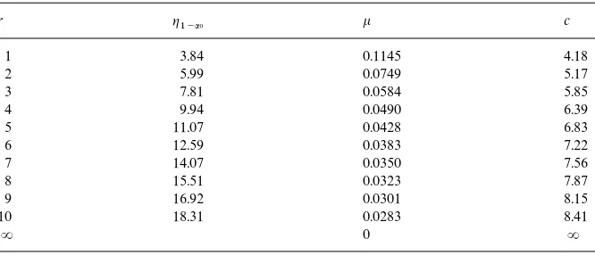
Table 1 presents the implied c values for e"5%, maxbias"$0.5% and

a₀"5%.

By regressing logkvs. logrand for the case of a nominal levela₀"5% at the model, one can obtain the simple approximation

c+3

e r0.3(maxbias)1@2. (35)

We now come back to the robustness of e$ciency properties of a GMM test and

"rst investigate the case of a GMM speci"cation test. Let

(P_g!-5_,_n)

n|N:"

AA

1!

g

Jn

B

Ph0

# g

Jn Ph1

B

_n_|N

(36)

be a sequence of local alternatives toP

h0 and

U

e,n(Pg!-5,n) :"

G

P1e,n,Q:"

A

1! e

JnBPg!-5,n# e

Jn QDQ3dom(a8)

H

(37)

be the corresponding asymptotic neighborhood ofP_g!-5_,_n, for givenn.

A natural restriction on the magnitude of the contamination isDeD(_DgD. This allows us to distinguish the neighborhoodU

e,n(Pg!-5,n) of the local alternative from

(17)

a given neighborhood U

e0,n(Ph0) of the null hypothesis with a neighborhood U

e,n(Pg!-5,n) of the local alternative. In this case a natural restriction will be De₀D#DeD(DgD.

The next theorem is the &power' counterpart of Theorem 1 for the GMM speci"cation test. Similarly to the case of the level, the theorem yields an explicit asymptotic bound by which the maximal asymptotic bias of the power can be bounded.

denote bynthe power functional of the test based onmM.Let further(P1_e_,

n,Q)n|N be

a sequence of(e,n,Q)-contaminations of the underlying local alternativesP_g!-5_,_neach

of them belonging to a corresponding neighborhoodU

e,n(Pg!-5,n) as dexned in(37). Then

lim

n?= Dn(P1e,n,Q)

!_n(P_g!-5

,n)D"2keg

P

RN

IF?₍_x_; ;_M_, _P!-5

g,n) dQ(x)

]

P

RN

IF(x;;_M_, _P

h0) dPh1(x)#o(g) (38)

with k dexned as in Theorem 1. Moreover, the bias of the asymptotic power

functionalnis uniformly bounded by the inequality

lim

n?= Dn(P1e,n,Q)

!n(P_g!-5_,_n)D)2keg max

M_P!_g-5_,n_{_}_P_h₀N sup_x DDh(x;a8()))DD2W0#o(g). (39)

Similarly to the case for the level, the maximal asymptotic bias of the power of a GMM speci"cation test derived from the RGMM estimator of the last section can be estimated by the inequality

lim

n?= Dn(P1e,n,Q)

!n(P_g!-5_,_n)D)2kegc2#o(g). (40)

As in the case of the level (see (33)) this inequality can be used to relate the tuning constantcof our RGMM estimator to the maximal bias in the power of the GMM speci"cation test, given a nominal levela₀ at the model. For instance, assumingH!k"1 ande"5%, a bound of 0.5% on the bias from a nominal level of 5% impliesc"4.18 andk"0.1145 (cf. Table 1). This yields an absolute maximal bias in the power of a corresponding RGMM speci"cation test given by 0.20g. For example forg"15% the implied maximal bias in the power is approximatively 3%.

Theorem 2 illustrates the trade o! existing between power and robustness of a GMM speci"cation test. Indeed, for a given maximal bias over the contaminated neighborhoodU

e,n(Pg!-5,n) one cannot impose stronger robustness

(18)

Table 1

Values of the tuning constantcfor bounding the maximal bias of the level of a GMM test!

r g_1~_a₀ k c

1 3.84 0.1145 4.18

2 5.99 0.0749 5.17

3 7.81 0.0584 5.85

4 9.94 0.0490 6.39

5 11.07 0.0428 6.83

6 12.59 0.0383 7.22

7 14.07 0.0350 7.56

8 15.51 0.0323 7.87

9 16.92 0.0301 8.15

10 18.31 0.0283 8.41

R 0 R

!The values of the tuning constantcare for a nominal level 5% at the model, for a maximal bias given bymaxbias"$0.5% and for a model contaminatione"5%.ris the number of degrees of freedom implied by thes2-test under scrutiny.

direction P_h

1 (that is with a higher constant g). On the other side, imposing

stronger robustness requirements by a lower constantcreduces the maximal bias from the power of the given local alternativeP_g!-5_,_n. However, for near local alternatives (and therefore low values ofg) this will correspond to a low power of the RGMM speci"cation test over the full contaminated neighborhood

U

e,_{We conclude this section by discussing the robustness of e}n(Pg!-5,n). _$_{ciency properties}

of the GMM-based Wald, score, and likelihood ratio tests. Consider again the neighborhood de"ned by (31). For P_e0_,_n_,_Q3U

e,n(Ph0) we de"ne a sequence of

parametric local alternatives to (24) by

g

A

a(h₀)# D

JnB"0 (41)

with a non-zero vectorD3Rk.

Similarly to the case of the GMM speci"cation test, a natural restriction on the magnitude of the contamination isDeD(DD_D_{. This allows us to distinguish the}

neighborhoodU

e,n(Ph0) of the local alternative from the given null hypothesis.

The next theorem is the power counterpart of Theorem 1 for the maximum-likelihood-type GMM tests. Similarly to Theorem 2 an explicit asymptotic bound for the maximal bias in the power of a parametric GMM test is provided.

(19)

Then the bias ofnis uniformly bounded by the inequality

lim

n?=Dn(P0e,n,Q)

!n(P

h0)D)2keDDDDDR~10 sup

x DDh(x; a(h0))DDw0

#o(D), (42)

wherek is dexned as in Theorem 1.

Similarly to the case for the power of a GMM speci"cation test, the maximal asymptotic bias of the power of a parametric GMM test derived from the RGMM estimator of the last section can be estimated by the inequality

lim

n?=Dn(P0e,n,Q)

!n(P

h0)D)2keDDDDDR~10 c#o(D). (43)

This bound can be used to relate the choice ofcto the maximal bias in the power of a parametric GMM test, given a nominal valuea₀ at the model.

5. An application to RGMM testing for conditional heteroscedasticity

In this section we consider a simple application of our RGMM methodology to a test for ARCH structures in the errors of a linear autoregressive model. The goal is not to perform a full analysis of the robustness properties of ARCH testing procedures but to outline the performance of the RGMM in a simple application as well as the algorithm used to compute the RGMM estimator of Section 3.

Let (y

t)t|Nbe the autoregressive process (1) with ARCH(1) error terms pres-ented in Example 2. Moreover, consider the orthogonality conditions given by (2) and (3).

A test for a constant conditional variance speci"cation ofe

tcould be a Hansen

speci"cation test for the overidentifying orthogonality conditions implied by the null hypothesisa₁"0 against an alternative hypothesisa₁'0.

Note that in the present formulation we treat all parameters that have to be estimated under the null hypothesis symmetrically. Of course, one could easily develop a two-stage RGMM testing procedure if (b₀, b₁) is treated as a vector of nuisance parameters.

To construct a GMM test for conditional heteroscedasticity behaving satis-factorily under local deviations from normality, we consider as a reference model fory

t an autoregressive model with normally distributed errors ut and

(20)

To compare the performance of the given GMM and RGMM tests for ARCH we simulate the following distributions&near'the normal distribution as candi-date models of a possible data generating process foru

t.

1. Standard normal.

In this experiment we compare the e$ciency of the RGMM and the classical GMM testing procedures at the given reference model.

2. Contaminated normalCN(e,K2).

F(x)"(1!_e)U₍_x₎#_eU

A

x

K

B

, x3R, (44)

whereUis the cumulative distribution function of a standard normal random variable. Here, we investigate the performance of the classical GMM and the RGMM under a known maximum distance e from the standard normal model and a given degree of contaminating varianceK2. We simulate this case for a distance e"0.05 and a very high contaminating variance

K2"100. This choice is quite extreme. However, it allows us to compare the performances of the RGMM and the GMM under dramatic symmetric deviations from normality that could occur over a short time period in real data.

3. Studentt_l withldegrees of freedom.

We consider the casesl"5, 9 that allow for the existence of the fourth and the eighth conditional moments of u

t, respectively. Note that the t9 and t

5distributions are already very near to the normal. As a consequence, in this

example we can compare the numerical performance of the robust and the classical GMM when very small deviations from normality are present. Moreover, in thet

5case we can investigate the impact of the non-existence of

some theoretical conditional moments ofu

t (assumed"nite by the GMM).

4. Double exponential DE.

This distribution has a symmetric convex density. It is therefore qualitat-ively di!erent from the normal already in the center of the distribution. Furthermore, it displays fat tails somewhere between the t

5 and the CN(0.05, 102) distribution.

All simulated error distributions were scaled in order to have variance 1. This small simulation design covers a good spectrum of tail behaviors for distribu-tions of u

t that have heavier tails than the normal and still satisfy minimal

moment requirements. Indeed, the tail indices (cf. Gasko and Rosenberger, 1983, p. 322) of these distributions are 1 for the standard normal distribution, 1.16 and 1.34 for the Student t

9 and t5 distributions, respectively, 1.63 for the double

(21)

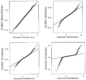
9All QQ plots are based on simulated samples of 5000 observations. Fig. 1. QQ Plot of the unconditional distribution of (y

t) (sample size 5000 observations) under

standard normal,t

5, double exponential and contaminated normal (e"0.05,K"10) errors. The

ARCH parameter was set toa

1"0.

We simulate (1) for the parameter choice (b₀,b₁,a₀)"(0.4, 0.3, 0.25) and for di!erent values ofa₁, ranging from 0 to 0.3, under the di!erent distributions foru

t presented above and for sample sizes¹"250, 500, 1000. Note that for a₁'1

3the fourth unconditional moments ofutdo not exist even under

normal-ity ofu

t.

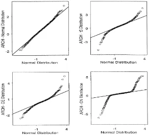
As an illustration, some QQ plots9 of the unconditional distribution of a process (y

t) without and with ARCH e!ects (a1"0 anda1"0.2, respectively)

for some of the distributions considered above are presented in Figs. 1 and 2. From these graphs one can see that the e!ects on the unconditional distribu-tion ofy

t of a&slight' modi"cation of the conditional distribution ofut can be

(22)

Fig. 2. QQ Plot of the unconditional distribution of (y

t) (sample size 5000 observations) under

standard normal,t

5, double exponential and contaminated normal (e"0.05,K"10) errors. The

ARCH parameter was set toa

1"0.2.

distribution for u

t induce fatter tails in the unconditional distributions of

y

t_{Each model is simulated 1000 times. The corresponding empirical rejection}when ARCH structures are present.

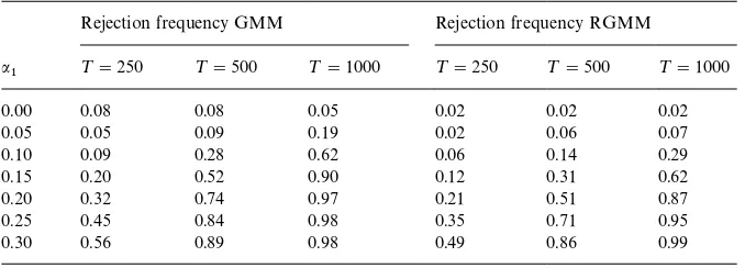
frequency for the RGMM and the GMM Hansen's test is calculated for a"xed nominal level of 5%. The estimated standard error of the empirical rejection frequencyp( is given by (using the binomial distribution) ((p((1!p())/1000)1@2. It is 0.7%, 1.0% and 1.5% forp("5%, 20%, 50%, respectively.

The tuning constant for the RGMME was set at c"2.09. This allows to obtain a maximal bias of $0.5% in the level of the RGMM test also for contaminationse"10% (cf. Table 1 above) of the unconditional distribution of

y

t. We imposed such a strong robustness restriction on our RGMME because

the unconditional distribution ofy

tshows even fatter tails than the conditional

distribution of u

t when ARCH e!ects are present, a fact that can make the

distance between the induced unconditional distributions ofy

t larger than the

distance between the assumed conditional distributions ofu

(23)

Table 2

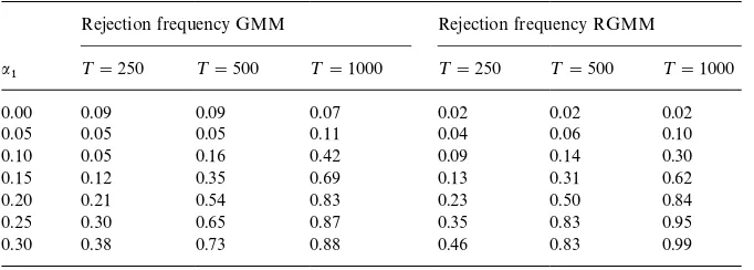
GMM and RGMM simulation results underu

t&N(0, 1)!

Rejection frequency GMM Rejection frequency RGMM

a

1 ¹"250 ¹"500 ¹"1000 ¹"250 ¹"500 ¹"1000

0.00 0.08 0.08 0.05 0.02 0.02 0.02

0.05 0.05 0.09 0.19 0.02 0.06 0.07

0.10 0.09 0.28 0.62 0.06 0.14 0.29

0.15 0.20 0.52 0.90 0.12 0.31 0.62

0.20 0.32 0.74 0.97 0.21 0.51 0.87

0.25 0.45 0.84 0.98 0.35 0.71 0.95

0.30 0.56 0.89 0.98 0.49 0.86 0.99

!Each entry in the table corresponds to the empirical rejection frequency of the hypothesisa₁"0 obtained using 5% critical values for thes2test. The constantcfor the RGMM test was set to c"2.09.

For each simulation run we useda

0"(0.2, 0.2, 0.2) as a starting point for the

algorithm and always obtained convergence.

In the "rst step of the algorithm we set q"0 and updated the matrix A

after having estimated the covariance matrix of h(X

1,a0) with a Newey and

West (1987b) covariance matrix estimator. In the second step of the algorithm we simulated an ARCH process corresponding to the parameter choice a

0

and computed the expectations needed to solve (22) and thereby obtain q₁.

A₁ is obtained after having estimated the covariance matrix of (h(X₁, a₀)!_q

0)wc(A0(h(X1, a0)!q0)) with a Newey and West (1987b)

covariance matrix estimator. Note that at this stage of the algorithm an autocor-relation robust covariance matrix estimator is necessary even when (h(X

t,a0))t|N is conditionally uncorrelated because this does not generally imply that (hA0,q0

c (Xt, a0))t|N is uncorrelated. In the third step we computed the GMME

a

1 associated to the orthogonality function hAc1,q1. The second and third step

above are then iterated until convergence of the sequence (a

n)n|N of GMME associated to the sequence (hAn,qn

c )n|NH of bounded orthogonality functions.

The results are presented in Tables 2}6. Although the goal of this simulation is not to perform a full analysis of the robustness properties of ARCH testing procedures, some of the features obtained are worth noting.

First of all, the RGMM test yields empirical sizes that are very stable across all simulated distributions (generally between 0.02 and 0.03). On the other side, the empirical sizes of the classical GMM tests are far less stable ranging between 0.05 (for the normal distribution and for a sample size¹"1000) and 0.11 (in some experiments with theDEand t

5 distributions) for distributions that are

(24)

Table 3

t&DE!

a

1 ¹"250 ¹"500 ¹"1000 ¹"250 ¹"500 ¹"1000

0.00 0.11 0.10 0.09 0.03 0.03 0.03

0.05 0.04 0.04 0.09 0.03 0.06 0.12

0.10 0.04 0.12 0.31 0.07 0.14 0.32

0.15 0.06 0.23 0.54 0.11 0.26 0.58

0.20 0.10 0.33 0.71 0.18 0.41 0.78

0.25 0.16 0.43 0.78 0.26 0.57 0.91

0.30 0.21 0.50 0.79 0.34 0.70 0.96

Table 4

t&t9!

a

1 ¹"250 ¹"500 ¹"1000 ¹"250 ¹"500 ¹"1000

0.00 0.09 0.09 0.07 0.02 0.02 0.02

0.05 0.05 0.05 0.11 0.04 0.06 0.10

0.10 0.05 0.16 0.42 0.09 0.14 0.30

0.15 0.12 0.35 0.69 0.13 0.31 0.62

0.20 0.21 0.54 0.83 0.23 0.50 0.84

0.25 0.30 0.65 0.87 0.35 0.83 0.95

0.30 0.38 0.73 0.88 0.46 0.83 0.99

too limited to draw "nal conclusions, we observe empirical sizes re#ecting a rather&conservative'behavior of the RGMM test and a drastic liberal behav-ior of the classical GMM test. Indeed, already under normality the empirical sizes of the classical GMM test are often higher than the given nominal level of 5% (for sample sizes¹"250, 500).

Secondly, the RGMM test yields empirical power curves that are fairly stable for almost all the simulated distributions. In particular, for distributions that are not &too far' from the normal (the DE, the t

9 and the t5 distributions) the

(25)

Table 5

t&t5!

a

1 ¹"250 ¹"500 ¹"1000 ¹"250 ¹"500 ¹"1000

0.00 0.10 0.11 0.11 0.02 0.02 0.03

0.05 0.05 0.05 0.06 0.03 0.07 0.11

0.10 0.06 0.10 0.24 0.05 0.14 0.33

0.15 0.11 0.18 0.43 0.11 0.28 0.61

0.20 0.15 0.29 0.59 0.17 0.46 0.82

0.25 0.21 0.40 0.67 0.29 0.64 0.93

0.30 0.27 0.48 0.71 0.40 0.78 0.97

Table 6

t&CN(0.05, 10)!

a

1 ¹"250 ¹"500 ¹"1000 ¹"250 ¹"500 ¹"1000

0.00 0.35 0.51 0.48 0.02 0.01 0.02

0.05 0.16 0.19 0.17 0.02 0.03 0.06

0.10 0.09 0.08 0.05 0.03 0.06 0.14

0.15 0.06 0.04 0.02 0.06 0.11 0.24

0.20 0.04 0.03 0.03 0.07 0.16 0.36

0.25 0.04 0.03 0.06 0.10 0.22 0.48

0.30 0.04 0.04 0.11 0.13 0.28 0.60

normality by no more than$0.09 (with a maximal absolute deviation of 0.09 obtained for the DE case when a₁"0.2). In the contaminated normal case di!erences are larger. However, note that in this case the classical GMM test does not even produce a monotonically increasing power curve.

(26)

classical and robust power curves in thet

9 experiment are quite comparable,

with some small advantages for the GMM (RGMM) for large (small) sample sizes. For larger deviations, (thet

5, theDEand theCNcase) the power of the

RGMM is clearly higher than that of the classical test. This suggests that in real data applications already very small contaminations of the underlying model could a!ect the e$ciency of classical GMM testing procedures. On the other side, a RGMM procedure could then be helpful in maintaining this e$ciency loss below a given bound.

6. Conclusions

We derived a RGMM estimator that generates robust tests for a broad class of GMM test statistics. Special cases are Hansen's speci"cation test and likeli-hood-type GMM tests like the Wald, the score and the likelihood ratio test.

We presented an algorithm to compute our RGMM estimator, in which the degree of robustness required by a researcher can be controlled through the choice of an appropriate tuning constantc.

We explicitly related the choice of this tuning constant to two key variables: the amount of contamination that one can realistically assume with respect to a given data set and to the available data information, and the maximal bias of level and (or) power of a GMM test that one is ready to admit for the given test. In some simulated experiments we presented evidence that the optimal performance of a GMM test at the model can be strongly worsened even when small deviations are present. In these experiments the RGMM testing procedure behaves well in controlling small distributional deviations from the assump-tions. Moreover, the e$ciency loss at the model of the RGMM procedure seems to be reasonable when considering its performance under small model mis-speci"cations.

Further research on RGMM testing includes the study of its performance under more general model structures and model deviations (for instance asym-metric deviations) than those presented above. Applications to more complex macroeconomic and "nancial models where a reference model for the data distribution can be assumed could produce interesting robust results that can be compared with those obtained with classical methodologies. Finally, a further issue is the small sample behavior of RGMM statistics.

Acknowledgements

(27)

10See Clarke (1986), Bednarski (1993) and Heritier and Ronchetti (1994).

Appendix A

A.1. Proof of Theorem 1

We prove the statement of the theorem only for the score and likelihood ratio statistics. Those formM andmWcan be proved by similar arguments. As noted after Property 1a8 is FreHchet di!erentiable.10This implies the FreHchet di! erenti-ability of;_S_{. A}_"_{rst-order Von Mises (1947) expansion of};_S_{then gives up to}

terms of order o(e)

Jn(;S₍_P

hn)!;S(P0e,n,Q))PN(0,Ir), nPR (A.1) in distribution uniformly for allQ3dom(;_S_{), using (30). As shown by Heritier}

and Ronchetti (1994) the asymptotic level under contamination of the corre-sponding symmetric test functional induced by;_S_{can be then approximated by}

the second-order expansion given by (32) with;";_S_{. Note that the equality}

forkin the statement of the theorem is obtained by a result of Johnson and Kotz (1991), Chapter 28, p. 132, formula 1. Then, by (4) and using the hypothesis

g(a(P

h0))"0, we obtain

IF(x; ;_S_, _P

h0)"R1@20 Eh0

Lh?₍_X

1; a(h0))

La =0

]

A

E_h 0

Lh(X 1;a(h0))

La? IF(x;a(, Ph₀)#h(x; a(h₀))

B

.

The constrained GMM estimator (a((P_h

n), jK(Phn)) is de"ned by the system of

"rst-order conditions

E_h

n

Lh?₍_X

1;a((Phn))

La =nEhnh(X1;a((Phn))!

Lg?

La(a((Phn))jK(Phn)"0

g(a((P_h

n))"0,

where jK :dom(jK)PRr is the corresponding statistical functional of Lagrange multipliers. Di!erentiating implicitly the limit version of these necessary condi-tions in directiond

x3dom(a()}while imposing (4) andjK(Ph0)"0}and solving

the corresponding system of implicit equations gives

IF(x; a(, P

(28)

where

Inserting this result in (A.2) and using (14) with=

0"<0~1yields

Moreover, by the orthogonal projection property ofM

0R0(with respect to the

This proves the theorem foraS.

To apply the approximation (32) to the likelihood-ratio statistic remember thata8 is FreHchet di!erentiable. A second-order von Mises (1947) expansion of

mRunder the hypotheses (4) andg(a(P_h This expression can be simpli"ed by using (A.2), (14) with=

0"<0~1, and the

orthogonal projection property of M

0R0 (with respect to the scalar product

(29)

The expression on the right-hand side of this formula is the second-order von Mises expansion under the hypotheses (4) and g(a(P

h0))"0 of a (cf. Hausman, 1978; Holly, 1982). As a consequence the di!erence between the levels under contamination of the likelihood ratio test and a Hausman test de"ned by the critical region MnmH(P

hn)*g1~a0N, where g1~a0 is the 1!a0

quantile of as2(r, 0) distribution, is of order o(e2). Hence, the asymptotic bias under a givenP0_e_,

n,Q-contamination of the level of the likelihood ratio test can be

equivalently investigated by analyzing that of the Hausman test. Similar argu-ments to those developed above for ;S_{can be now applied to} ;H_{. The IF of}

using (A.2) and (14). Furthermore, again by the properties of orthogonal projec-tions, this quantity can be bounded by the self-standardized norm of h as follows:

(30)

Some calculations then yield

h0)"0. This concludes the proof of the theorem. h

A.3. Proof of Theorem 3

The functional;_W _{is asymptotically equivalent to};_S_and;_R_{at the model}

under the local alternatives given by (41); cf. Gourieroux and Monfort (1989). Moreover the FreHchet di!erentiability of a8 implies that this equivalence is uniform. It is therefore su$cient to prove the theorem for the functional

;W_{. The statistic} _n_mW₍_P

Similar calculations to those in the proof of Theorem 2 then give

(31)

Expanding;W₍_P

The Cauchy}Schwarz inequality then gives

KA

Ln(P_>,0_n_,_Q)

Using again the properties of orthogonal projections we obtain

KA

Ln(P0_>,

n,Q)

Le

K

_e_/0

BK

)2ksup_x DDh(x; a(h0))DDW0DDDDDR~10 #o(D). (A.10)

Finally, by inserting this expression in the Taylor expansion (A.7) we get

Dn(P0_e_,

n,Q)!n(Ph0)D)2keDDDDDR~10 sup

x DDh(x;a(h0)DDW0

#o(D). (A.11)

(32)

References

Amemiya, T., 1974. The nonlinear two-stages least squares estimator. Journal of Econometrics 2, 105}110.

Bansal, R., Hsieh, D., Viswanathan, S., 1993. No arbitrage and arbitrage pricing: a new approach. Journal of Finance 48, 1719}1747.

Bednarski, T., 1993. FreHchet di!erentiability of statistical functionals and implications to robust statistics. In: Morgenthaler, S., Ronchetti, E., Stahel, W. (Eds.), New Directions in Statistical Data Analysis and Robustness. BirkhaKuser, Basel, pp. 26}34.

Clarke, B.R., 1986. Nonsmooth analysis and FreHchet di!erentiability of M-functionals. Probability Theory and Related Fields 73, 197}209.

Engle, R.F., 1982. Autoregressive conditional heteroscedasticity with estimates of the variance of United Kingdom in#ation. Econometrica 50, 987}1007.

Gasko, M., Rosenberger, J.L., 1983. Comparing location estimators: means, medians, and trimean. In: Hoaglin, D.C., Mosteller, F., Tukey, J.W. (Eds.), Understanding Robust and Exploratory Data Analysis. Wiley, New York, pp. 297}338.

Gourieroux, C., Monfort, A., 1989. A general framework for testing a null hypothesis in a mixed form. Econometric Theory 5, 63}82.

Hampel, F.R., 1968. Contribution to the theory of robust estimation. Ph.D. Thesis, University of California, Berkeley.

Hampel, F.R., 1974. The in#uence curve and its role in robust estimation. Journal of the American Statistical Association 69, 383}393.

Hampel, F.R., Ronchetti, E.M., Rousseeuw, P.J., Stahel, W.A., 1986. Robust Statistics: The Ap-proach Based on In#uence Functions. Wiley, New York.

Hansen, L.P., 1982. Large sample properties of generalized method of moments estimators. Econo-metrica 50, 1029}1054.

Hausman, J.A., 1978. Speci"cation tests in econometrics. Econometrica 46, 1251}1272.

Heritier, S., Ronchetti, E., 1994. Robust bounded-in#uence tests in general parametric models. Journal of the American Statistical Association 89, 897}904.

Holly, A., 1982. A remark on Hausman's speci"cation tests. Econometrica 50, 749}759. Huber, P., 1981. Robust Statistics. Wiley, New York.

Imbens, G.W., Spady, R.H., Johnson, P., 1998. Information theoretic approaches to inference in moment condition models. Econometrica 66, 333}357.

Johnson, N., Kotz, S., 1991. Continuous and Discrete Distributions, Vol. 2. Wiley, New York. Koenker, R.W., 1982. Robust methods in econometrics. Econometric Review 1, 213}255. Koenker, R.W., Bassett, G., 1978. Regression quantiles. Econometrica 46, 33}50.

Koenker, R.W., Machado, J.A.F., 1999. GMM inference when the number of orthogonality condi-tions is large. Journal of Econometrics 93, 327}344.

Koenker, R.W., Machado, J.A.F., Skeels, C.L., Welsh, A.H., 1994. Momentary lapses: moment expansions and the robustness of minimum distance estimation. Econometric Theory 10, 172}197.

Krasker, W.S., 1986. Two-stage bounded-in#uence estimators for simultaneous equations models. Journal of Business and Economic Statistics 4, 437}444.

Krasker, W.S., Welsch, R.E., 1985. Resistant estimation for simultaneous-equations models using weighted instrumental variables. Econometrica 53, 1475}1488.

Krishnakumar, J., Ronchetti, E., 1997. Robust-estimators for simultaneous equations models. Journal of Econometrics 78, 295}314.

KuKnsch, H., 1984. In"nitesimal robustness for autoregressive processes. Annals of Statistics 12, 843}863.

(33)

Markatou, M., Ronchetti, E., 1997. Robust inference: the approach based on in#uence functions. In: Maddala, G.S., Rao, C.R. (Eds.), Handbook of Statistics, Vol. 15. North-Holland, Amsterdam, pp. 49}75.

Martin, R.D., Yohai, V.J., 1986. In#uence functionals for times series. Annals of Statistics 14, 781}818.

Newey, W.K., 1985. Generalized method of moments speci"cations testing. Journal of Econometrics 29, 229}256.

Newey, W.K., West, K.D., 1987a. Hypothesis testing with e$cient method of moments estimation. International Economic Review 28, 777}787.

Newey, W.K., West, K.D., 1987b. A simple positive-de"nite, heteroscedasticity and autocorrelation consistent covariance matrix estimator. Econometrica 55, 703}708.

Peracchi, F., 1990. Robust M-estimators. Econometric Review 9, 1}30. Peracchi, F., 1991. Robust M-tests. Econometric Theory 7, 69}84.

Rousseeuw, P.J., Leroy, A., 1987. Robust-Regression and Outlier Detection. Wiley, New York. Von Mises, R., 1947. On the asymptotic distribution of di!erentiable statistical functions. Annals of