FDD Massive MIMO Channel Estimation with
Arbitrary 2D-Array Geometry
Jisheng Dai, An Liu, and Vincent K. N. Lau
Abstract—This paper addresses the problem of downlink chan-nel estimation in frequency-division duplexing (FDD) massive multiple-input multiple-output (MIMO) systems. The existing methods usually exploit hidden sparsity under a discrete Fourier transform (DFT) basis to estimate the cdownlink channel. How-ever, there are at least two shortcomings of these DFT-based methods: 1) they are applicable to uniform linear arrays (ULAs) only, since the DFT basis requires a special structure of ULAs; and 2) they always suffer from a performance loss due to the leakage of energy over some DFT bins. To deal with the above shortcomings, we introduce an off-grid model for downlink channel sparse representation with arbitrary 2D-array antenna geometry, and propose an efficient sparse Bayesian learning (SBL) approach for the sparse channel recovery and off-grid refinement. The main idea of the proposed off-grid method is to consider the sampled grid points as adjustable parameters. Utilizing an in-exact block majorization-minimization (MM) algorithm, the grid points are refined iteratively to minimize the off-grid gap. Finally, we further extend the solution to uplink-aided channel estimation by exploiting the angular reciprocity between downlink and uplink channels, which brings enhanced recovery performance.
Index Terms—Channel estimation, massive multiple-input multiple-output (MIMO), sparse Bayesian learning (SBL), majorization-minimization (MM), off-grid refinement.
I. INTRODUCTION
Massive multiple-input multiple-output (MIMO) has at-tracted significant attention in wireless communications, and has been widely considered as a key candidate technology to meet the capacity demand in 5G wireless networks [1], [2]. To fully reap the benefit of excessive base station (BS) antennas, knowledge of channel state information at the transmitter (CSIT) is essentially required [3]. Many research efforts have been devoted to time-division duplexing (TDD) massive MIMO, because the CSIT in the TDD mode can be obtained by exploiting channel reciprocity, where the pilot-aided training overhead is proportional to the number of active mobile users (MUs) only [4], [5]. However, in the frequency-division duplexing (FDD) mode, the conventional training overhead for the CSIT acquisition grows proportionally with the BS antenna size [6], [7], which can be quite large in massive MIMO systems. Hence, it appears to be an extremely challenging task to obtain accurate CSIT in FDD massive MIMO systems.
Fortunately, due to the limited local scattering effect in the propagation environment, the elements in the massive MIMO
The authors are with the Department of Electronic and Computer Engi-neering (ECE), Hong Kong University of Science and Technology (HKUST), Hong Kong (e-mail: [email protected]; [email protected]; [email protected]). J. Dai is also with the Department of Electronic Engineering, Jiangsu University, Zhenjiang 212013, China.
channel are highly correlated. Many works have shown that the effective dimension of a massive MIMO channel is much less than its original dimension [8]–[11]. Specifically, if the BS is equipped with a large uniform linear array (ULA), the massive MIMO channel has an approximately sparse representation under the discrete Fourier transform (DFT) basis [10], [12], [13]. Exploiting such hidden sparsity, many efficient downlink channel estimation and feedback algorithms have been proposed in recent years [8], [10], [11], [14]–[19]. Nevertheless, it is worth noting that the validity of the DFT basis as a sparse representation of a massive MIMO channel depends on ULAs. When the antenna geometry deviates from a ULA, the aforementioned methods will fail to work.
DFT-based channel estimation methods always have a per-formance loss, even for ULA systems, because of the leakage of energy in the DFT basis. As shown in [20]–[22], the DFT basis actually provides a fixed sampling grid that discretely covers the angular domain of the massive MIMO system. Since signals usually come from random directions, the leak-age energy caused by direction mismatch is unavoidable. To achieve a better sparse representation, Ding and Rao [20]–[22] considered an overcomplete DFT basis, which corresponds to a denser sampling grid on the angular domain. The overcomplete DFT method can alleviate the direction mismatch issue, but cannot fully eliminate it. When a coarse grid is used, the overcomplete DFT basis may still lead to a high direction mismatch. On the other hand, if a very dense sampling grid is used, thel1-norm-based recovery methods may not work well
due to high correlation between the basis vectors. To over-come the leakage issue and to generalize for general antenna geometry, dictionary learning techniques were also proposed in [20]–[22]. However, the standard dictionary learning approach has several drawbacks: 1) its convergence is not theoretically guaranteed; and 2) learning a comprehensive dictionary re-quires collecting a large amount of channel measurements as training samples from all locations in a specific cell, which may pose great challenges in practical implementations.
In this paper, we consider a generic off-grid model for channel sparse representation of massive MIMO systems with an arbitrary 2D-array geometry, and we propose an efficient sparse Bayesian learning (SBL) approach [23], [24] for joint sparse channel recovery and off-grid refinement. The main idea of the proposed method is to consider the sampled grid points as adjustable parameters. Then, we utilize an in-exact block majorization-minimization (MM) algorithm [25], [26] to refine the grid points iteratively. After several iterations, the refined points will converge to the actual directions of ar-rival/departure, so the proposed method can eliminate direction
mismatch in the angular domain. The following summarizes the contributions of this paper.
• Model-based Off-Grid Sparse Basis
We provide a novel off-grid model for massive MIMO channel sparse representation with an arbitrary 2D-array geometry. Off-grid models have been applied widely to the direction-of-arrival in array signal processing [27]– [29]. However, they do not work well in 2D massive MIMO channels. Different from the commonly used linear approximation off-grid model, the proposed model can fully eliminate the direction mismatch, rather than only alleviate the modeling error.
• Joint Sparse Channel Recovery and Off-Grid Refine-ment with Autonomous Learning
We propose an SBL-based framework based on in-exact block MM algorithm for joint sparse channel recovery and off-grid refinement. The proposed solution outper-forms l1-norm recovery [30]–[32],1 and has an inherent
learning capability, so no prior knowledge about the sparsity level, noise variance or direction mismatch is required. We show that the solution converges to the stationary solution of the optimization problem. Simu-lation results reveal substantial performance gains over the existing state-of-the-art baselines.
• Enhanced Recovery Performance with Angular Reci-procity
We further extend the solution to uplink-aided channel estimation by exploiting angular reciprocity2 between
downlink and uplink channels. Characterizing the joint sparse structure with angular reciprocity was first ad-dressed in [22]. However, it always has a performance loss due to the fact that the joint sparse structure only holds approximately. Our new extension strictly charac-terizes the joint sparse structure by the inherent mecha-nism of the off-grid model, bringing enhanced recovery performance.
The rest of the paper is organized as follows. In Section II, we present the system model and review the state-of-the-art DFT-based channel estimation for massive MIMO systems. In Section III, we provide the SBL-based off-grid method for downlink channel estimation. In Section IV, we extend the solution to exploit angular reciprocity. Numerical experiments and discussions follow in Sections V and VI, respectively.
N otations : C denotes complex number, k · kp denotes p-norm,(·)T denotes transpose,(·)H denotes Hermitian
trans-pose, (·)† denotes pseudoinverse, I denotes identity matrix,
AΩ denotes the sub-matrix formed by collecting the columns
from Ω, CN(·,µ,Σ) denotes complex Gaussian distribution with mean µand varianceΣ,supp(·) denotes the set of
in-1SBL methods includel
1-norm-based methods as a special case when a
maximum a posteriori(MAP) optimal estimate is adopted with a fixed Laplace signal prior, and theoretical and empirical results show that SBL methods with better priors can achieve enhanced performance over the l1
-norm-based methods [24], [33].
2We consider an FDD system, so the reciprocity of the channel realization
between the uplink and downlink does not hold. However, the directions of arrival and departure of the uplink are reciprocal with those of the downlink due to the fact that both the uplink and downlink face the same scattering structure [22].
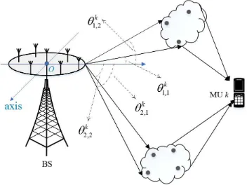
Fig. 1. Illustration of downlink channel model for a massive MIMO system withNc=Ns= 2.
dices of nonzero elements,Vec(·)denotes vectorization,tr(·)
denotes trace operator, diag(·) denotes diagonal operator, ⊙ denotes Hadamard product, and⊗denotes Kronecker product.
II. MASSIVEMIMO CHANNELMODEL ANDEXISTING SOLUTIONS
A. Massive MIMO Channel Model
Consider a massive MIMO system operating in FDD mode. There is one BS withN(≫1)antennas andKMUs equipped with a single antenna. The array at the BS has an arbitrary geometry in the plane. Without loss of generality, we define the origin of a polar coordinate system to be at the first element of the array, and denote the coordinates of the n-th sensor
(dn, φn), as illustrated in Fig. 1. We consider a flat fading
channel, and the downlink channel vector from the BS to the k-th user is given by [34], [35]
hk =
Nc
X
c=1
Ns
X
s=1
ξc,sk a(θkc,s), (1)
where Nc stands for the number of scattering clusters, Ns
stands for the number of sub-paths per scattering cluster,ξk c,s
is the complex gain of thes-th sub-path in thec-th scattering cluster for thek-th MU, andθk
c,sis the corresponding azimuth
angle-of-departure (AoD). The steering vector a(θ)∈CN×1
is
a(θ) = [e−j2π d1
λdϕ1(θ), e−j2π d2
λdϕ2(θ), . . . , e−j2π dN
λdϕN(θ)
]T,
(2)
whereϕn(θ) = sin(θ−φn), andλd is the wavelength of the
downlink propagation. For a ULA,a(θ)can be simplified by
a(θ) = [1, e−j2π d
λdsin(θ), . . . , e−j2π
(N−1)d
λd sin(θ)]T, (3)
wheredstands for the distance between adjacent sensors. According to the geometry-based stochastic channel model (GSCM) [36], the number of scattering clustersNc is usually
B. Review of Downlink Channel Estimation
In this subsection, we review the state-of-the-art DFT-based sparse channel estimation for the downlink channel in an FDD system. Assume that the BS is equipped with a ULA, and it broadcasts a sequence ofT training pilot symbols, denoted by X∈CT×N, for each MU to estimate the downlink channel.
Then, the downlink received signal yk ∈ CT×1 at the k-th
MU is given by
yk =Xhk+nk, (4)
where nk ∈CT×1 stands for the additive complex Gaussian
noise with each element being zero mean and varianceσ2 in
the downlink, and tr(XXH) =P T N with P/σ2 measuring
the training SNR. Since the number of antennasNat the BS is large, it is unlikely to obtain a robust recovery ofhk by using
conventional channel estimation techniques, e.g., least squares (LS) method. Recently, the emerging compressed sensing (CS) technique has given new interest in the problem of downlink channel estimation with limited training overhead. The main idea of these methods is to find a sparse representation ofhk
in the DFT basis [34], i.e.,
hk =Ftk (5)
whereF∈CN×N denotes the DFT matrix andt
kis the sparse
representation channel vector. Then, the received signalyk in (4) can be formulated as
yk =XFtk+nk, (6)
and the corresponding sparse signal recovery problem is given by
min
tk k
tkk0, subject tokyk−XFtkk2≤ǫ, (7)
whereǫis a constant determined by the upper bound ofknkk2.
Asl0-norm is non-convex, it is usually relaxed byl1-norm, i.e.,
min
tk k
tkk1, subject tokyk−XFtkk2≤ǫ. (8)
C. Challenges for the DFT-based Method
In this subsection, we discuss challenges for the DFT-based method. Firstly, this method is applicable to ULAs only, which is explained as follows. The DFT matrix can be written in the form of
which provides a fixed grid that uniformly covers the range [−1
3. As illustrated in
(3), the steering vectors of ULAs share the same structure with f(x). For each sampling point (e.g., the n-th point), we can always find a θˆn in the angular domain such that
d
λdsin(ˆθn) = −
1 2 +
n−1
N . Hence, it is equivalent to saying
3Only the firstNpoints are used in the DFT matrix sincef(
−12) =f(12).
the DFT basis actually provides a fixed sampling grid in the angular domain. When the true AoDs θk
c,ss lie on (or,
practically, close to) the sampling points {θˆ1,θˆ2, . . . ,θˆN+1},
the channel vector hk definitely has a sparse representation
in the DFT basis. Since the sparse property hinges strongly on the shared structure between the DFT basis and the ULA steering, the DFT-based method is applicable to ULAs only.
The other shortcoming of the DFT-based method is that it always has a performance loss, even for ULA systems, due to the leakage of energy. As will be illustrated shortly, the leakage of energy caused by direction mismatch is unavoidable in practice. According to (5), we have
tk=FHhk=
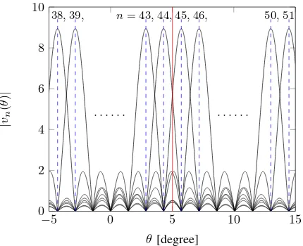
is no energy leakage. In practice, however, direction mismatch is unavoidable because signals usually come from random directions. Any direction mismatch will result in the leakage of energy in the DFT basis. Fig. 2 shows an example of the energy leakage, where the ULA is of size N = 80 and the inter-antenna spacing is a half wavelength. For an off grid AoD (e.g, θ∗ = 5.0198◦), there is a very serious energy leakage,
where both|v44(θ∗)| and|v45(θ∗)| have large values, as well
as some significant values with|v43(θ∗)|and|v46(θ∗)|.
To achieve a better sparse representation, [20]–[22] applied an overcomplete DFT basis, which corresponds to a denser sampling grid covering the angular domain with more points. Note that the overcomplete DFT method can alleviate the direction mismatch, but cannot fully eliminate it. In order to solve the problem of direction mismatch, as well as extend the sparse channel estimation method to more general array geometry, we propose an efficient SBL-based off-grid method for downlink channel estimation with an arbitrary 2D-array geometry. The main idea of the proposed method is to consider the sampled grid points as the adjustable parameters. Then, we utilize an in-exact block MM algorithm to iteratively refine the grid points. After several iterations, the refined points will converge to the true directions, so the proposed method can better eliminate the direction mismatch in the angular domain.
−5 0 5 10 15 0
2 4 6 8 10
38,39, n= 43,44,45,46, 50,51,
· · · ·
θ [degree]
|
vn
(
θ
)
|
Fig. 2. Illustration of problem of energy leakage for the DFT basis, where the sampling points for the DFT basis in the angular domain are denoted by the dotted blue lines, the true AoD atθ = 5.0198◦is denoted by the red line, and the distance between the red line and the nearest dotted blue line is called the direction mismatch.
2D-array geometry. For ease of exposition, we proceed as follows. We begin by introducing a model-based off-grid basis to handle the direction mismatch for the 2D array with an arbitrary geometry. Then, we apply this off-grid model to the downlink channel estimation, an an in-exact MM algorithm is provided, as well as its convergence analysis.
A. Off-Grid Basis for Massive MIMO Channels
For ease of notation, we drop the MU’s indexkand denote the true AoDs as{θl, l= 1,2, . . . , L}, whereL=NcNs. Let
ˆ
ϑ ={ϑˆl}
ˆ
L
l=1 be a fixed sampling grid that uniformly covers
the angular domain[−π
2,π2], whereLˆ denotes the number of
grid points. If the grid is fine enough such that all the true DOAsθls,l= 1,2, . . . , L, lie on (or practically close to) the
grid, we can use the following model for h:
h=Aw, (13)
where A =
a( ˆϑ1), a( ˆϑ2), . . . , a( ˆϑLˆ)
∈ CN×Lˆ, a(θ)
is a steering vector for a 2D array with a known arbitrary geometry [defined in (2)], and w ∈ CLˆ×1 is a sparse vector
whose non-zero elements correspond to the true directions at
{θl, l = 1,2, . . . , L}. For example, if the ˆl-th element of w
is nonzero and the corresponding true direction isθl, then we
haveθl= ˆϑˆl. Note that the DFT basis becomes a special case
of A if the BS is equipped with a ULA and the number of grid points is set toLˆ =N.
As mentioned in Section II-B, the assumption of the true directions being located on the predefined spatial grid is usually invalid in practice. To handle the direction mismatch, we adopt an off-grid model. Specifically, ifθl∈ {/ ϑˆi}
ˆ
L
i=1 and
ˆ
ϑnl, nl ∈ {1,2, . . . ,Lˆ}, is the nearest grid point to θl, we writeθl as
θl= ˆϑnl+βnl, (14)
where βnl corresponds to the off-grid gap. Using (14), we havea(θl) =a( ˆϑnl+βnl). Then,hcan be rewritten as
h=A(β)w, (15)
where β = [β1, β2, . . . , βLˆ]T, A(β) = [a( ˆϑ1+β1),a( ˆϑ2+
β2), . . . ,a( ˆϑLˆ+βLˆ)], and
βnl =
(
θl−ϑˆnl, l= 1,2, . . . , L
0, otherwise .
Note that with the off-grid basis, it is possible to fully eliminate the direction mismatch because there always exists some βnl making (14) hold exactly. The received signalyin (6) can be rewritten by
y=XA(β)w+n=Φ(β)w+n, (16)
where Φ(β) , XA(β). Since the coefficient vector β is unknown, the currentl1-norm minimization algorithm can not
be applied to the off-grid channel model (16) directly. To jointly recover the sparse signal and refine the grid points, we adopt the SBL algorithm [23], [24], which is one of the most popular approaches for sparse recovery and perturbation calibration. Theoretical and empirical results show that SBL methods can achieve enhanced performance over l1
regular-ized optimization (please also refer to our simulations). In the following, we will discuss how to jointly recover the sparse signal and refine the grid.
B. Sparse Bayesian Learning Formulation
Under the assumption of circular symmetric complex Gaus-sian noises, we have
p(y|w, α,β) =CN(y|Φ(β)w, α−1I), (17)
where α = σ−2 stands for the noise precision. Since α is
usually unknown, we model it as a Gamma hyperpriorp(α) = Γ(α;a, b), where we seta=b=ǫ(ǫ >0 is a small number, e.g., ǫ = 0.0001) as in [23], [24] so as to obtain a broad hyperprior. We assume a noninformative uniform prior forβ. Following the commonly used sparse Bayesian model [23], we further assign a non-stationary Gaussian prior distribution with a distinct precision γi for each element of w. Letting
γ= [γ1, γ2, . . . , γLˆ]T, we have
p(w|γ) =CN(w|0,diag(γ−1)). (18)
Similarly, we modelγis as independent Gamma distributions,
i.e.,
p(γ) = ˆ
L Y
i=1
Γ(γi;a, b). (19)
This two-stage hierarchical prior gives
p(w) =
Z ∞
0 CN
(w|0,diag(γ−1))p(γ)dγ
∝ ˆ
L Y
i=1
b+|wi|2
−(a+12),
which is recognized as encouraging sparsity due to the heavy tails and sharp peak at zero with a smallb[23], [33]. In fact, it can be shown that finding a MAP estimate ofwwith the prior (20) is equivalent to finding the minimum l0-norm solution
using FOCUSS with p → 0 [37]. This explains why SBL methods can achieve enhanced performance over thel1
-norm-based methods. Since directly finding the aforementioned MAP estimate ofwis difficult, SBL methods introduce a two-stage hierarchical prior to get around the problematic MAP estimate. We refer interested readers to Section V of [33] for details.
It is worth noting that the precisionsγls in (18) fully indicate
the support of w. For example, ifγlis large, the l-th element
of w tends to zero; otherwise, the value of the l-th element is significant. As a consequence, once we obtain the precision vectorγ, as well as the off-grid gapβ, the estimated downlink channel hecan be obtained by
he=AΩ(β) (ΦΩ(β))†y, (21)
whereΩ = supp(w). Therefore, in the rest part of this section, we only need to focus on finding the optimalγandβ. As the noise precision αis still unknown, we find the most-probable values α⋆,γ⋆ andβ⋆ together by maximizing the posteriori
p(α,γ,β|y), i.e.,
(α⋆,γ⋆,β⋆) = arg max
α,γ,βp(α,γ,β|y), (22)
or, equivalently,
(α⋆,γ⋆,β⋆) = arg max
α,γ,βlnp(y, α,γ,β). (23)
The above objective is a high-dimensional non-convex func-tion. It is difficult to directly use the gradient ascent method on the original objective function because gradient ascent is known to have a slow convergence speed, and moreover, the gradient of the original objective function has no closed-form expression. To overcome this challenge, we propose a novel in-exact block MM algorithm to find a stationary point of (23).
C. Overview of the In-exact Block MM Algorithm
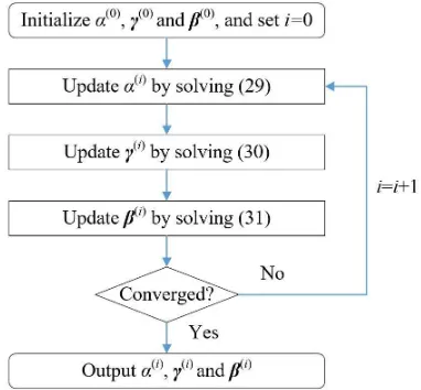
The principle behind the block MM algorithm is to itera-tively construct a continuous surrogate function (lower bound) for the objective functionlnp(y, α,γ,β), and then alternately maximize the surrogate function with respect to α, γ and
β. The surrogate function is chosen such that the alternating maximization w.r.t. each variable has a closed-form/simple solution.
Specifically, letU(α,γ,β|α,˙ γ˙,β˙)be the surrogate function constructed at some fixed point ( ˙α,γ˙,β˙) which satisfies the
Fig. 3. The overall flow of the block MM algorithm.
following properties:
U(α,γ,β|α,˙ γ˙,β˙)≤lnp(y, α,γ,β), ∀α,γ,β, (24)
U( ˙α,γ˙,β˙|α,˙ γ˙,β˙) = lnp(y,α,˙ γ˙,β˙), (25) ∂U(α,γ˙,β˙|α,˙ γ˙,β˙)
∂α
α= ˙α
= ∂lnp(y, α,γ˙,β˙)
∂α
α= ˙α
, (26)
∂U( ˙α,γ,β˙|α,˙ γ˙,β˙)
∂γ
γ= ˙γ
= ∂lnp(y,α,˙ γ,β˙)
∂γ
γ= ˙γ , (27)
∂U( ˙α,γ˙,β|α,˙ γ˙,β˙)
∂β
β= ˙β
= ∂lnp(y,α,˙ γ˙,β)
∂β
β= ˙β . (28)
Then, we updateα,γ,β as
α(i+1)= arg max
α U(α,γ
(i),β(i)
|α(i),γ(i),β(i)), (29)
γ(i+1)= arg max
γ U(α
(i+1),γ,β(i)
|α(i+1),γ(i),β(i)), (30)
β(i+1)= arg max
β U(α
(i+1),γ(i+1),β
|α(i+1),γ(i+1),β(i)), (31)
where(·)(i)stands for thei-th iteration. The overall flow of the
block MM algorithm is given in Fig. 3. The update rules (29)– (31) guarantee the convergence of the block MM algorithm as follows.
Lemma 1.The update rules (29)–(31) give a non-decreasing sequencelnp(y, α(i),γ(i),β(i)),i= 1,2,3, . . .
Proof:See Appendix A.
In the block MM algorithm, we need to obtain the optimal solutions for the maximization problems in (29)–(31). How-ever, the maximization problem w.r.t.βin (31) is non-convex and it is difficult to find its optimal solution. Therefore, in this paper, we use an in-exact MM algorithm where β(i+1)
D. Detailed Implementations
To update α, γ and β, we first have to choose an ap-propriate surrogate function U(α,γ,β|·,·,·) that satisfies the properties mentioned in (24)–(28). Inspired by the expectation-maximization (EM) algorithm [38], we use the corresponding lower bound function as the surrogate function; i.e., for any fixed point( ˙α,γ˙,β˙), we construct the surrogate function as
U(α,γ,β|α,˙ γ˙,β˙)
=
Z
p(w|y,α,˙ γ˙,β˙) lnp(w,y, α,γ,β)
p(w|y,α,˙ γ˙,β˙)dw, (32)
and we have the following lemma.
Lemma 2. All the properties in (24)–(28) hold true with the surrogate functionU(α,γ,β|·,·,·)given in (32).
Proof: See Appendix B.
Note that, from (17) and (18), p(w|y, α,γ,β) is complex Gaussian [23], [27]:
p(w|y, α,γ,β) =CN(w|µ(α,γ,β),Σ(α,γ,β)), (33)
where
µ(α,γ,β) =αΣ(α,γ,β)ΦH(β)yk,
Σ(α,γ,β) = αΦH(β)Φ(β) + diag(γ)−1 .
With U(α,γ,β|·,·,·), we discuss the hyperparameter up-dates for α,γ andβ, respectively, as follows.
1) Update forα: The maximization problem in (29) has a simple and closed-form solution:
Lemma 3. The optimization problem (29) has a unique solution:
α(i+1)= T+a
b+η(α(i),γ(i),β(i)), (34)
where
η(α,γ,β) = tr Φ(β)Σ(α,γ,β)ΦH(β)
+ky−Φ(β)µ(α,γ,β)k22.
Proof: See Appendix C.
2) Update forγ: The maximization problem in (30) also has a simple and closed-form solution:
Lemma 4. The optimization problem (31) has a unique solution:
γl(i+1)= a+ 1
b+
Ξ(α(i+1),γ(i),β(i)) ll
, ∀l, (35)
where
Ξ(α,γ,β) =Σ(α,γ,β) +µ(α,γ,β)µH(α,γ,β).
Proof: See Appendix D.
3) Update forβ: Since the maximization problem (31) is non-convex and it is difficult to find its optimal solution, we apply gradient update on the objective function of (31) and obtain a simple one-step update forβ. We name the procedure of updating β as grid refining, because it is related with the modeling error caused by the off-grid gap. The derivative of the objective function in (31) w.r.t. β can be calculated as
ζ(i)= [ζ(i)(β1), ζ(i)(β2), . . . , ζ(i)(β ˆ
L)]
T, (36)
with
ζ(i)(β
l) =2Re
(a′( ˆϑl+βl))HXHX(a( ˆϑl+βl))
·c(1i)
+ 2Re(a′( ˆϑl+βl))HXHc
(i) 2
, (37)
where c(1i) = −α(i+1)(χ (i)
ll + |µ
(i)
l |
2), c(i)
2 =
α(i+1)((µ(i)
l )∗y
(i) −l − X
P j6=lχ
(i)
jl a( ˆϑj + βj)), y
(i) −l =
y−X·P j6=l(µ
(i)
j ·a( ˆϑj+βj)),a′( ˆϑj+βl) =da( ˆϑj+βl)/dβl,
µl(i)andχjl(i)denote thel-th element and the(j, l)-th element of µ(α(i+1),γ(i+1),β(i)) and Σ(α(i+1),γ(i+1),β(i)),
respectively. The detailed derivation for (37) can be found in Appendix E. It is clear that the optimal solution for β is hard to obtain. Fortunately, due to the convergence property illustrated in (72), we just have to find a suboptimal solution that increases the value of the objective function step by step. The most popular numerical method is to update the value of βl in the derivative direction, i.e.,
β(i+1)=β(i)+ ∆β·ζ(i), (38)
where∆βis the stepsize. Here, we can resort to backtracking
line search [39] to determine the maximum stepsize∆β, which
ensures that the objective value can be strictly decreased before reaching the stationary point.
E. Convergence Analysis and Discussion
From Lemma 1, the sequence lnp(y, α(i),γ(i),β(i)), i = 1,2,3, . . ., is non-decreasing and it converges to a limit because the evidence function has the upper bound of 1. In the following, we further prove that the sequence of iterates generated by the algorithm converges to a stationary point.
Theorem 5.For the surrogate function defined in (32), if vari-ables are iteratively updated by (34), (35) and (38), the iterates generated by the in-exact block MM algorithm converge to a stationary solution of the optimization problem (23).
Proof:See Appendix F.
Next, we address the difference between the proposed in-exact block MM algorithm and the EM algorithm. The original SBL method usually exploits the EM algorithm to perform the Bayesian inference. The EM algorithm iteratively constructs the same lower bound as in (32), and simultaneously updates α,γ andβ by
(α(i+1),γ(i+1),β(i+1)) = arg max
α,γ,βU(α,γ,β|y, α
(i),γ(i),β(i)).
(39)
The EM algorithm can find a local optimal solution and its convergence can be guaranteed, if the joint maximization problem in (39) is solvable. Unfortunately, in our problem, (39) is non-convex and is intractable in the presence of β. Hence, the EM algorithm cannot be directly applied to our problem.
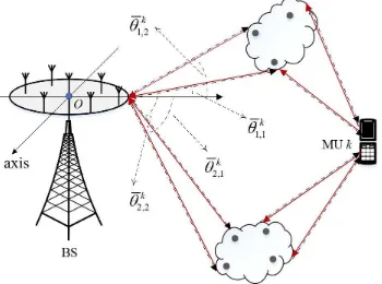
Fig. 4. Illustration of angular reciprocity for a massive MIMO system with
Nc=Ns= 2, where the downlink transmission and the uplink transmission
are denoted by dotted black line and red line, respectively.
by replacing the steering vectora(θl) =a( ˆϑnl+βnl)with the linear approximation
a(θl)≈a( ˆϑnl) +βnl·a
′( ˆϑ
nl), (40)
the surrogate function in (32) becomes convex and thus can be maximized efficiently. However, we do not adopt this linear approximation method, because the modeling error caused by the off-grid gap cannot be fully eliminated. Particularly, if a coarse grid is used, (40) may still lead to a large modeling error, and the final channel estimation performance will be poor.
IV. CHANNELESTIMATION WITHANGULARRECIPROCITY For the downlink channel estimation, the training period T could become a bottleneck of the recovery performance, because the dimension of the measurement vectoryin (16) is determined by the training periodT, whileT is usually much less thanN. The performance of the downlink channel estima-tion can be improved if we collect more useful informaestima-tion. Inspired by the angular reciprocity used in [22], we extend the off-grid method to uplink-AoA-aided channel estimation in this section. Note that angular reciprocity is quite different from the commonly used channel reciprocity in TDD systems. In the first subsection, we will explain angular reciprocity in detail.
A. Angular Reciprocity
Following the downlink channel model in Section II-A, the uplink channel vector from the k-th user to the BS is given by
¯
hk= Nc
X
c=1
Ns
X
s=1 ¯
ξk
c,s¯a(¯θc,sk ), (41)
whereξ¯k
c,sis similarly defined asξc,sk ,θ¯kc,sis the corresponding
azimuth angle-of-arrival (AoA), as illustrated in Fig. 4, and the steering vectora¯(θ)∈CN×1 is
¯
a(θ) = [e−j2π d1
λuϕ1(θ), e−j2π
d2
λuϕ2(θ), . . . , e−j2πdNλuϕN(θ)
]T,
where λu is the wavelength of uplink propagation. Usually,
channel reciprocity does not hold in FDD systems because
different frequency bands are used in the downlink and uplink transmission. However, if the downlink and uplink transmis-sions operate closely in time, it is reasonable to have the following assumption:
Assumption 6 (Angular Reciprocity [22]). The AoAs of signals for the k-the MU in the uplink transmission almost coincide with the AoDs of signals in the downlink transmis-sion, i.e.,
θk
c,s= ¯θkc,s, ∀k, c, s, (42)
as illustrated in Fig. 4.
To exploit the angular reciprocity, Ding and Rao [22] collected the downlink and uplink channel vectors for thek-th MU in pair
hk=Ftk, (43)
¯
hk=F¯tk, (44)
where ¯tk is the sparse representation of h¯k under the DFT
basis for ULAs. It is worth noting that the steering vectors a(θk
c,s) and a¯(¯θc,sk ) are distinct if different frequency bands
are used. Hence, the angular reciprocity between the downlink and uplink transmissions does not bring a joint sparse structure for tk and¯tk. To get around this problem, they assume that
the frequency duplex distance is not large (i.e., λd ≈λu). In
this case, they approximately have
a(θk
c,s)≈a¯(¯θc,sk ), (45)
and then
supp(tk)≈supp(tk). (46)
As the joint sparse structure only holds approximately, it may results in performance loss. To handle this drawback, we will propose a joint off-grid model in the next subsection.
B. Joint Off-Grid Model
For the uplink channel estimation, assume that each MU broadcasts a sequence of T¯ training pilot symbols, denoted by sk ∈ CT¯×1, k = 1,2, . . . , K. Then, the received signal
¯
Y∈CN×T¯ at the BS is given by
¯
Y= ¯HS+ ¯N, (47)
where H¯ = [¯h1,h¯2, . . . ,h¯K] ∈ CN×K with h¯k being the
channel vector for the k-th MU, S = [s1,s2, . . . ,sK]T ∈
CK×T¯, and N¯ ∈ CN×T¯ stands for the additive complex
Gaussian noise with each element being zero mean and varianceσ¯2in the uplink. If the number of MUs is small, i.e.,
K≤T, the uplink channel matrix¯ Hu can be easily obtained by the conventional LS estimate, i.e.,
[¯hls1,h¯ls2, . . . ,h¯lsK],YS¯ † = ¯H+E,
(48)
or, equivalently,
¯
hlsk =¯hk+ek, k= 1,2, . . . , K, (49)
where h¯ls
k stands for the LS estimate of h¯k and E ,
[e1,e2, . . . ,eK]stands for the estimation error. IfSconsists of
with the requirement T ≥ N for the downlink channel estimation, it is much easier to meet the requirement T¯≥K for the uplink channel estimation.
With (49) and (16), we are able to exploit the sparse property of each MU independently. We drop the MU’s index kfor ease of notation, and then the paired sparse representation equalities can be rewritten as
y=Φ(β)w+n, (50)
¯
hls= ¯Φ(β) ¯w+e, (51)
where (50) coincides with (16), Φ¯(β) = [¯a( ˆϑ1+β1),¯a( ˆϑ2+
β2), . . . ,¯a( ˆϑLˆ + βLˆ)], and w¯ is the sparse representation
of h¯ls. If the angular reciprocity holds, it is easy to check that supp(w) = supp( ¯w). Different from the approximation method [22] that hinges on the condition of (45), our off-grid model guarantees a jointly sparse structure from the angular domain directly, where neither approximation ofλd≈λu nor
the assumption of ULA at the BS is required. In the following, we will show how to jointly recover the sparse vectorswand
¯
w in the framework of SBL with the in-exact MM algorithm. Since the results can be similarly derived by following the procedures in Section III, detailed derivations are omitted for brevity.
C. Sparse Bayesian Learning Formulation
Under the assumption of circular symmetric complex Gaus-sian noises, we have
p(y|w, α,β) =CN(y|Φ(β)w, α−1I), (52) p(¯hls|w,¯ α,¯ β) =CN(¯hls|Φ¯(β) ¯w,α¯−1I), (53)
whereα¯ stands for the noise precision of e, which is further modeled as a Gamma hyperprior p(¯α) = Γ(¯α; a, b). Recall that, in Section III-B, we have used γ to control the sparsity of w as follows:
p(w|γ) =CN(w|0,diag(γ−1)). (54)
If we letτ = [τ1, τ2, . . . , τLˆ]T be a nonnegative vector and
p( ¯w|γ) =CN( ¯w|0,diag((γ⊙τ)−1)), (55)
wandw¯ will share a joint sparse structure. For example,γl−1 tends to zero, so is (γlτl)−1. Therefore, (54) and (55) provide
a mathematic representation of the angular reciprocity. The estimated uplink channelh¯ls contains the AoA information in
the uplink. The proposed method only exploits the AoA infor-mation in h¯ls to help in identifying the AoD in the downlink
(downlink channel support) via the angular reciprocity in (54) and (55). The small scale fading information contained in the estimated uplink channel h¯ls cannot be exploited since the
channel reciprocity does not hold for FDD systems.
D. Bayesian Inference
For ease of notation, let wa , {w,w¯}, ya , {y,h¯ls},
Θ , {α,α,¯ γ,τ,β}. We assume a noninformative uniform
prior for τ. At some fixed point Θ =˙ {α,˙ α,˙¯ γ˙,τ˙,β˙}, we construct the surrogate function as
U(Θ|Θ) =˙
Z
p(wa|ya,Θ) ln˙ p(w
a,ya,Θ)
p(wa|ya,Θ)˙ dw
a, (56)
where
p(wa,ya,Θ) =p(y|w, α,β)p(w|γ)p(¯hls|w,¯ α,¯ β) ·p( ¯w|γ,τ)p(α)p(¯α)p(γ)p(τ)p(β)
and
p(wa|ya,Θ) =CN(w|µ(α,γ,β),Σ(α,γ,β)) · CN( ¯w|µ¯(¯α,γ,τ,β),Σ¯( ¯α,γ,τ,β)), with
¯
µ(¯α,γ,τ,β)) = ¯αΣ¯Φ¯H(β)¯hls,
¯
Σ(¯α,γ,τ,β)) = ¯αΦ¯H(β) ¯Φ(β) + diag(γ⊙τ)−1 .
Note thatµ(α,γ,β)andΣ(α,γ,β)have been defined in (33). In the maximization step of the (i+ 1)-th iteration, we updateα,α,¯ γ,τ,β as
α(i+1)= arg max
α U(α,α¯
(i),
γ(i),τ(i),β(i)|Θ(i)),
(57)
¯
α(i+1)= arg max ¯
α U(α
(i+1),α,¯ γ(i),τ(i),β(i)
|Θ(1i)), (58)
γ(i+1)= arg max
γ U(α
(i+1),α¯(i+1),γ,τ(i),β(i)
|Θ(2i)), (59)
τ(i+1)= arg max
τ U(α
(i+1),α¯(i+1),
γ(i+1),τ,β(i)|Θ(3i)),
(60)
β(i+1)= arg max
β U(α
(i+1),α¯(i+1),γ(i+1),τ(i+1),β |Θ(4i)).
(61)
whereΘ(ji) denotes the first j elements of Θ(i) coming from
the(i+1)-th iteration. Extending Lemmas 3 and 4, the updates for α,α,¯ γ andτ can be obtained as follows:
Corollary 7. The optimization problems (57)–(60) have unique solutions:
α(i+1)= T +a
b+ηd(Θ(i))
, (62)
¯
α(i+1)= N+a
b+ηu(Θ
(i) 1 )
, (63)
γ(li+1)= a+ 2
b+hΞd(Θ(2i)) +τlΞu(Θ
(i) 2 )
i
ll
, ∀l, (64)
τl(i+1)=h 1 γl(i+1)Ξu(Θ(3i))
i
ll
, ∀l, (65)
where
ηd(Θ) = tr Φ(β)Σ(α,γ,β)ΦH(β)
+ky−Φ(β)µ(α,γ,β)k22,
ηu(Θ) = tr ¯Φ(β) ¯Σ(¯α,γ,τ,β) ¯ΦH(β)
+
h¯ls−Φ¯(β)¯µ(¯α,γ,τ,β)
2 2,
Ξd(Θ) =Σ(α,γ,β) +µ(α,γ,β)µH(α,γ,β),
Proof: The proof is omitted for brevity.
In the following, we discuss how to refine the grid for the uplink-AoA-aided channel estimation. Ignoring the terms independent ofβ, the objective function in (61) becomes
U(α(i+1),α¯(i+1),γ(i+1),τ(i+1),β
Finally, we updateβ in the derivative direction, i.e.,
β(i+1)=β(i)+ ∆β·ζ(i), (68)
and resort to backtracking line search to determine the max-imum stepsize ∆β. Since the optimization problems (57)–
(60) have unique solutions (Corollary 7), it can be similarly proved to Theorem 5 that the uplink-AoA-aided method also converges to a stationary solution.
V. SIMULATIONRESULTS
In this section, we conduct simulations to investigate the performance of our proposed methods. The proposed methods are compared with the classical DFT method, the original SBL method, the overcomplete DFT method, and the dictionary learning method. We use the 3GPP spatial channel model (SCM) [35] to generate the channel coefficients for an urban microcell. Since the state-of-the-art methods, as well as the SCM, work for ULAs only, the results for non-ULAs are not reported here. The uplink frequency is1980MHz, the down-link frequency is2170MHz, and the inter-antenna spacing is
d=c/(2f0), withcbeing the light speed andf0= 2000MHz.
The normalized mean square error (NMSE) is defined as
1
mis the estimate ofhmat then-th Monte Carlo trial
andMc = 200is the number of Monte Carlo trials.
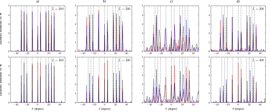
A. Recovered Channel Sparsity in the Angular Domain
In Fig. 5, we illustrate the effect of direction mismatch on the channel sparse representation performance for different channel estimation strategies. Consider a simple scenario where a ULA with100antennas at the BS is used to send the training pilot symbols with ten AoDs in total, which are simply denoted as θ1=−30◦, θ2=−25◦, θ3=−20◦,θ4 =−10◦,
θ5 = 0◦, θ6 = 5◦, θ7 = 15◦, θ8 = 20◦, θ9 = 25◦, and
θ10 = 30◦. The training pilots are randomly generated with
T = 40and the SNR is set to10dB. Fig. 5 shows the element modulus of the recovered channel sparse representation w, where the number of grid pointsLˆ is fixed to200 or 400for all the methods, except for the classical DFT method. It is observed that 1) the solution of the classical DFT method is not exactly sparse, and it has a significant performance loss due to the leakage of energy over many bins; 2) the original SBL method and the overcomplete DFT method can achieve better sparse representations, especially for a dense grid (Lˆ = 400), but direction mismatch always exists; and 3) our proposed off-grid method can greatly improve the sparsity and accuracy of the channel representation, and the direction mismatch can be almost eliminated.
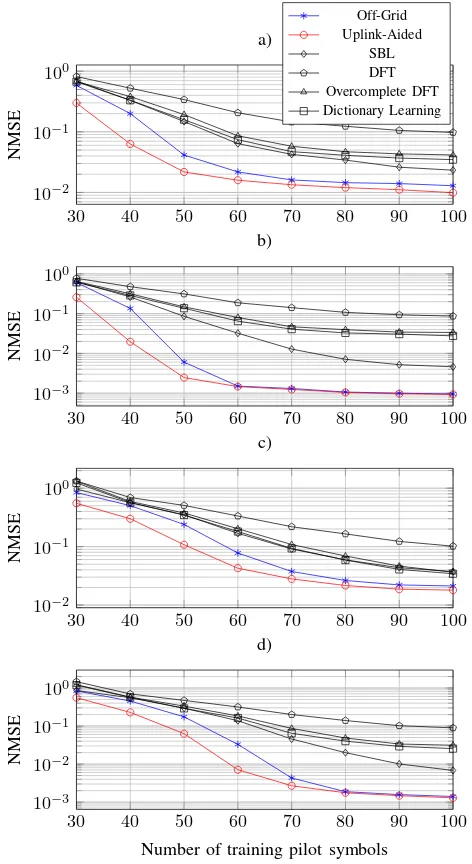
B. Channel Estimation Performance VersusT
In Fig. 6, Monte Carlo trials are carried out to investigate the impact of the number of pilot symbols on the downlink channel estimation performance. Assume that the ULA at the BS is equipped with 150 antennas, and the system supports ten MUs, where each MU has a single antenna. All the results are obtained by averaging over 200 Monte Carlo channel realizations. Every channel realization consists ofNc random
scattering clusters ranging from−40◦to40◦, and each cluster
contains Ns = 10 subpaths concentrated in a 20◦ angular
spread. The training pilots are randomly generated, the SNR is chosen as 0 dB or 10 dB, and the number of grid points is fixed to 200 for all but the DFT method. Fig. 6 shows the NMSE performance of the downlink channel estimate achieved by the different channel estimation strategies versus the number of training pilot symbols T, where the number of scattering clusters is set to Nc = 2 or Nc = 3. It can
−40 −20 0 20 40
Fig. 5. Element modulus ofwfor three independent trials withN = 100,T = 40and SNR= 10 dB. The true AoDs are denoted by dotted lines. a) Off-Grid; b) SBL; c) DFT; d) Overcomplete DFT.
improve the performance of the downlink channel estimation, as it collects more useful information than the off-grid method.
C. Channel Estimation Performance Versus Lˆ
In Fig. 7, we study the impact of the number of grid points on the downlink channel estimation performance. We consider the same scenario as in Section V-B, except for the number of training pilot symbols being fixed to 50or70. All the results are obtained by averaging over 200 Monte Carlo channel realizations. Fig. 7 shows the NMSE performance of the downlink channel estimate achieved by the different channel estimation strategies versus the number of grid points
ˆ
L. It is shown that the classical DFT method, the overcomplete DFT method and the original SBL method achieve the same performance atLˆ = 150, because they use the same grid in the case ofN = ˆL. The NMSE of our methods decreases as the number of grid points increases, and they always outperform the others, no matter what number of grid points is used.
D. Channel Estimation Performance VersusN
In Fig. 8, we study the channel estimation performance against the number of antennas at the BS. Here, we also consider the same scenario as in Section V-B, except for the number of grid points being fixed to 300. Fig. 8 shows the NMSE performance of the downlink channel estimate achieved by the different channel estimation strategies versus the number of antennas at the BS. Fig. 8 reaffirms that our methods can achieve the best performance compared with the state-of-art methods. It can be seen that 1) the NMSE of all the methods increases as the number of antennas increases, because the dimension of the unknown channel matrix become large, while the dimension of the pilots remains unchanged. 2) the classical DFT mehod, the overcomplete method and the original SBL method almost achieve the same performance at N = 300, because the grids coincide with each other whenLˆ=N; and 3) the uplink-CSI-aided method significantly improves the performance of downlink channel estimation, especially for smallN, because it utilizes moreN measurements than the off-grid method.
VI. CONCLUSION
The problem of downlink channel estimation in FDD mas-sive MIMO systems is addressed in this paper. We provide a novel off-grid model for massive MIMO channel sparse representation, which can greatly improve the sparsity and accuracy of the channel representation. To the best of our knowledge, our work is the first to utilize off-grid channel model to combat modeling error for channel estimation with an arbitrary 2D-array geometry. The proposed off-grid model and the SBL-based framework have wide applicability. They do not require any prior knowledge about the sparsity of channels, nor the variance of noises, and all the parameters are automatically tuned by the in-exact MM algorithm. Extending the results to MUs with multiple antennas is straightforward in the framework of SBL.
APPENDIX
A. Proof of Lemma 1
The non-decreasing property can be achieved as
30 40 50 60 70 80 90 100 10−2
10−1
100
NMSE
a)
Off-Grid Uplink-Aided
SBL DFT Overcomplete DFT Dictionary Learning
30 40 50 60 70 80 90 100
10−3
10−2
10−1
100
NMSE
b)
30 40 50 60 70 80 90 100
10−2
10−1
100
NMSE
c)
30 40 50 60 70 80 90 100
10−3
10−2
10−1
100
Number of training pilot symbols
NMSE
d)
Fig. 6. NMSE of dowlink channel estimate versus the number of training pilot symbols. a) Nc = 2, SNR= 0 dB; b)Nc = 2, SNR = 10dB; c)
Nc= 3, SNR= 0dB; d)Nc= 3, SNR= 10dB
B. Proof of Lemma 2
Letting q(w)be an arbitrary distribution, the lower bound of lnp(y, α,γ,β)can be written as
lnp(y, α,γ,β) = ln
Z
p(w,y, α,γ,β)dw
= ln
Z
q(w)p(w,y, α,γ,β)
q(w) dw
≥
Z
q(w) lnp(w,y, α,γ,β)
q(w) dw, (80)
where Jensen’s inequality is applied in the last step. The equality holds when p(w,y,α,q(w)γ,β) = c for a constant c that does not depend on w. As q(w) is a distribution, we have R
q(w)dw= 1. This further indicates that
c=
Z
p(w,y, α,γ,β)dw=p(y, α,γ,β) (81)
150 200 250 300 350 400
10−2
10−1
NMSE
a)
Off-Grid Uplink-Aided
SBL DFT Overcomplete DFT Dictionary Learning
150 200 250 300 350 400
10−2
10−1
Number of grid points
NMSE
b)
Fig. 7. NMSE of downlink channel estimate versus the number of grid points. a)Nc= 2,T = 50and SNR= 0dB; b)Nc= 3,T= 70and SNR
= 10dB.
100 150 200 250 300
10−2
10−1
100
NMSE
a)
Off-Grid Joint Off-Grid
SBL DFT Overcomplete DFT Dictionary Learning
100 150 200 250 300
10−2
10−1
100
Number of antennas at BS
NMSE
b)
Fig. 8. NMSE of dowlink channel estimate versus the number of antennas at BS with SNR= 10dB. a)Nc= 2andT = 40; b)Nc= 3andT= 60.
and
q(w) =p(w|y, α,γ,β). (82)
To prove (26), we first rewrite the left side of (26) as
On the other hand, the right side of (26) is
∂lnp(y, α,γ˙,β˙)
Combining (83) and (84), we achieve the equality in (26). Since the proofs for (27)–(28) can be similarly achieved, they are omitted for brevity.
C. Proof of Lemma 3
For α, ignoring the independent terms, the objective func-tion in (29) can be rewritten as
U(α,γ(i),β(i)|α(i),γ(i),β(i))
Since (85) is a strick concave function related toα, setting its derivative to zero gives the unique optimal solution
α(i+1)= T+a
b+η(α(i),γ(i),β(i)).
D. Proof of Lemma 4
For γ, ignoring the independent terms of the objective function in (30), we obtain
U(α(i+1),γ,β(i)|α(i+1),γ(i),β(i))
Differentiating w.r.t. eachγl yields
∂U(α(i+1),γ,β(i)
Then, setting the derivative to zero and solving forγlgive the
unique optimal solution
E. Derivation for Eq. (37)
Ignoring the independent terms, the objective function in (31) becomes
and
∂tr Φ(β)Σ(i)ΦH(β) ∂βl
=2Re(a′( ˆϑl+βl))HXHXa( ˆϑl+βl)
·χ(lli)
+ 2Re
(a′( ˆϑl+βl))HXHX· X
j6=l
χ(jli)a( ˆϑj+βj)
.
Hence, the derivative ofU(α(i+1),γ(i+1),β
|α(i+1),γ(i+1),β(i))
w.r.tβl is same as (37).
F. Proof of Theorem 5
According to Theorem 2-b in [25], the block MM algo-rithm will converge to a stationary solution if the following additional conditions are satisfied:
• All the properties in (24)–(28) hold true with the surro-gate function.
• At least two of the problems (29)–(31) have a unique solution.
Lemmas 2–4 guarantee that the above two conditions hold true, respectively
REFERENCES
[1] T. L. Marzetta, “Noncooperative cellular wireless with unlimited num-bers of base station antennas,”IEEE Trans. Wireless Commun., vol. 9, no. 11, pp. 3590–3600, 2010.
[2] F. Rusek, D. Persson, B. K. Lau, E. G. Larsson, T. L. Marzetta, O. Edfors, and F. Tufvesson, “Scaling up MIMO: Opportunities and challenges with very large arrays,”IEEE Signal Process. Mag., vol. 30, no. 1, pp. 40–60, 2013.
[3] J.-C. Shen, J. Zhang, K.-C. Chen, and K. B. Letaief, “High-dimensional CSI acquisition in massive MIMO: Sparsity-inspired approaches,”IEEE Systems Journal, vol. 11, no. 1, pp. 32–40, 2017.
[4] E. G. Larsson, O. Edfors, F. Tufvesson, and T. L. Marzetta, “Massive MIMO for next generation wireless systems,” IEEE Commun. Mag., vol. 52, no. 2, pp. 186–195, 2014.
[5] J. Hoydis, S. Ten Brink, and M. Debbah, “Massive MIMO in the UL/DL of cellular networks: How many antennas do we need?”IEEE J. Sel. Areas Commun., vol. 31, no. 2, pp. 160–171, 2013.
[6] B. Hassibi and B. M. Hochwald, “How much training is needed in multiple-antenna wireless links?”IEEE Trans. Infor. Theory, vol. 49, no. 4, pp. 951–963, 2003.
[7] L. Lu, G. Y. Li, A. L. Swindlehurst, A. Ashikhmin, and R. Zhang, “An overview of massive MIMO: Benefits and challenges,”IEEE J. Sel. Topics in Signal Process., vol. 8, no. 5, pp. 742–758, 2014. [8] Z. Gao, L. Dai, Z. Wang, and S. Chen, “Spatially common sparsity based
adaptive channel estimation and feedback for FDD massive MIMO,”
IEEE Trans. Signal Process., vol. 63, no. 23, pp. 6169–6183, 2015. [9] J. Hoydis, C. Hoek, T. Wild, and S. ten Brink, “Channel measurements
for large antenna arrays,” inInternational Symposium on ISWCS 2012. IEEE, 2012, pp. 811–815.
[10] X. Rao and V. K. Lau, “Distributed compressive CSIT estimation and feedback for FDD multi-user massive MIMO systems,”IEEE Trans. Signal Process., vol. 62, no. 12, pp. 3261–3271, 2014.
[11] Z. Gao, C. Zhang, Z. Wang, and S. Chen, “Priori-Information aided iterative hard threshold: A low-complexity high-accuracy compressive sensing based channel estimation for TDS-OFDM,”IEEE Trans. Wire-less Commun., vol. 14, no. 1, pp. 242–251, 2015.
[12] Z. Chen and C. Yang, “Pilot decontamination in wideband massive MIMO systems by exploiting channel sparsity,”IEEE Trans. Wireless Commun., vol. 15, no. 7, pp. 5087–5100, 2016.
[13] J.-C. Shen, J. Zhang, E. Alsusa, and K. B. Letaief, “Compressed CSI acquisition in FDD massive MIMO: How much training is needed?”
IEEE Trans. Wireless Commun., vol. 15, no. 6, pp. 4145–4156, 2016.
[14] X. Rao and V. K. Lau, “Compressive sensing with prior support quality information and application to massive MIMO channel estimation with temporal correlation,”IEEE Trans. Signal Process., vol. 63, no. 18, pp. 4914–4924, 2015.
[15] J. Choi, D. J. Love, and P. Bidigare, “Downlink training techniques for FDD massive MIMO systems: Open-loop and closed-loop training with memory,”IEEE J. Sel. Topics in Signal Process., vol. 8, no. 5, pp. 802–814, 2014.
[16] L. You, X. Gao, A. L. Swindlehurst, and W. Zhong, “Channel acquisition for massive MIMO-OFDM with adjustable phase shift pilots,” IEEE Trans. Signal Process., vol. 64, no. 6, pp. 1461–1476, 2016.
[17] Z. Gao, L. Dai, W. Dai, B. Shim, and Z. Wang, “Structured compressive sensing-based spatio-temporal joint channel estimation for FDD massive MIMO,”IEEE Trans. Commun., vol. 64, no. 2, pp. 601–617, 2016. [18] A. Liu, V. K. Lau, and W. Dai, “Exploiting burst-sparsity in massive
MIMO with partial channel support Information,”IEEE Trans. Wireless Commun., vol. 15, no. 11, pp. 7820–7830, 2016.
[19] A. Liu, F. Zhu, and V. K. Lau, “Closed-loop autonomous pilot and compressive CSIT feedback resource adaptation in multi-user FDD massive MIMO systems,”IEEE Trans. Signal Process., vol. 65, no. 1, pp. 173–183, 2017.
[20] Y. Ding and B. D. Rao, “Channel estimation using joint dictionary learning in FDD massive MIMO systems,” in IEEE GlobalSIP 2015. IEEE, 2015, pp. 185–189.
[21] ——, “Compressed downlink channel estimation based on dictionary learning in FDD massive MIMO systems,” inIEEE GLOBECOM 2015. IEEE, 2015, pp. 1–6.
[22] ——, “Dictionary learning based ssparse channel representation and estimation for FDD massive MIMO systems,” arXiv preprint arXiv:1612.06553, 2016.
[23] M. E. Tipping, “Sparse Bayesian learning and the relevance vector machine,”Journal of Machine Learning Research, vol. 1, no. Jun, pp. 211–244, 2001.
[24] S. Ji, Y. Xue, and L. Carin, “Bayesian compressive sensing,”IEEE Trans. Signal Process., vol. 56, no. 6, pp. 2346–2356, 2008.
[25] M. Razaviyayn, “Successive convex approximation: Analysis and appli-cations,” Ph.D. dissertation, University of Minnesota, 2014.
[26] Y. Sun, P. Babu, and D. P. Palomar, “Majorization-minimization algo-rithms in signal processing, communications, and machine learning,”
IEEE Trans. Signal Process., vol. 65, no. 3, pp. 794–816, 2017. [27] Z. Yang, L. Xie, and C. Zhang, “Off-grid direction of arrival estimation
using sparse Bayesian inference,”IEEE Trans. Signal Process., vol. 61, no. 1, pp. 38–43, 2013.
[28] Q. Liu, H. C. So, and Y. Gu, “Off-grid DOA estimation with nonconvex regularization via joint sparse representation,”Signal Process., 2017. [29] J. Dai, X. Bao, W. Xu, and C. Chang, “Root sparse Bayesian learning
for off-grid DOA estimation,” IEEE Signal Process. Letters, vol. 24, no. 1, pp. 46–50, 2017.
[30] D. Donoho and Y. Tsaig, “Fast solution of l1-norm minimization
problems when the solution may be sparse,”IEEE Trans. Informantion Theory, vol. 54, no. 11, pp. 4789–4812, 2008.
[31] D. L. Donoho, “Compressed sensing,”IEEE Trans. Infor. theory, vol. 52, no. 4, pp. 1289–1306, 2006.
[32] E. J. Cand`es, J. Romberg, and T. Tao, “Robust uncertainty principles: Exact signal reconstruction from highly incomplete frequency informa-tion,”IEEE Trans. Infor. Theory, vol. 52, no. 2, pp. 489–509, 2006. [33] D. P. Wipf and B. D. Rao, “Sparse Bayesian learning for basis selection,”
IEEE Trans. Signal Process., vol. 52, no. 8, pp. 2153–2164, 2004. [34] D. Tse and P. Viswanath, Fundamentals of Wireless Communication.
Cambridge university press, 2005.
[35] 3GPP, “Universal mobile telecommunications system (UMTS); Spatial channel model for multiple input multiple output (MIMO) simulations,”
3GPP TR 25.996 version 11.0.0 Release 11, 2012.
[36] A. F. Molisch, A. Kuchar, J. Laurila, K. Hugl, and R. Schmalenberger, “Geometry-based directional model for mobile radio channelsłprinci-ples and implementation,”Trans. Emerging TeleCommun. Technologies, vol. 14, no. 4, pp. 351–359, 2003.
[37] B. D. Rao and K. Kreutz-Delgado, “An affine scaling methodology for best basis selection,”IEEE Trans. Signal Process., vol. 47, no. 1, pp. 187–200, 1999.
[38] A. P. Dempster, N. M. Laird, and D. B. Rubin, “Maximum likelihood from incomplete data via the EM algorithm,” Journal of the Royal Statistical Society. Series B (Methodological), pp. 1–38, 1977. [39] S. J. Wright and J. Nocedal, “Numerical optimization,”Springer Science,