On Miura Transformations
and Volterra-Type Equations Associated
with the Adler–Bobenko–Suris Equations
Decio LEVI †, Matteo PETRERA ‡†, Christian SCIMITERNA‡† and Ravil YAMILOV §
† Dipartimento di Ingegneria Elettronica,Universit`a degli Studi Roma Tre and Sezione INFN,
Roma Tre, Via della Vasca Navale 84, 00146 Roma, Italy E-mail: [email protected]
‡ Dipartimento di Fisica E. Amaldi, Universit`a degli Studi Roma Tre and Sezione INFN,
Roma Tre, Via della Vasca Navale 84, 00146 Roma, Italy E-mail: [email protected], [email protected]
§ Ufa Institute of Mathematics, 112 Chernyshevsky Str., Ufa 450077, Russia
E-mail: [email protected]
Received August 29, 2008, in final form October 30, 2008; Published online November 08, 2008 Original article is available athttp://www.emis.de/journals/SIGMA/2008/077/
Abstract. We construct Miura transformations mapping the scalar spectral problems of the integrable lattice equations belonging to the Adler–Bobenko–Suris (ABS) list into the dis-crete Schr¨odinger spectral problem associated with Volterra-type equations. We show that the ABS equations correspond to B¨acklund transformations for some particular cases of the discrete Krichever–Novikov equation found by Yamilov (YdKN equation). This enables us to construct new generalized symmetries for the ABS equations. The same can be said about the generalizations of the ABS equations introduced by Tongas, Tsoubelis and Xenitidis. All of them generate B¨acklund transformations for the YdKN equation. The higher order generalized symmetries we construct in the present paper confirm their integrability.
Key words: Miura transformations; generalized symmetries; ABS lattice equations
2000 Mathematics Subject Classification: 37K10; 37L20; 39A05
1
Introduction
The discovery of new two-dimensional integrable partial difference equations (orZ2-lattice equa-tions) is always a very challenging problem as, by proper continuous limits, many other results on differential-difference and partial differential equations may be obtained. Moreover many physi-cal and biologiphysi-cal applications involve discrete systems, see for instance [13,25] and references therein.
In the present paper we shall consider the Adler–Bobenko–Suris (ABS) classification ofZ2 -lattice equations defined on the square -lattice [2]. We refer to the papers [3,24,28,17,18,27] for some recents results about these equations. Our main purpose is the analysis of their trans-formation properties. In fact, our aim is, on the one hand, to present new Miura transtrans-formations between the ABS equations and Volterra-type difference equations and on the other hand, to show that the ABS equations correspond to B¨acklund transformations for some particular cases of the discrete Krichever–Novikov equation found by Yamilov (YdKN equation) [30].
Section2is devoted to a short review of the integrableZ2-lattice equations derived in [2] and to present details on their matrix and scalar spectral problems. In Section3, by transforming the obtained scalar spectral problems into the discrete Schr¨odinger spectral problem associated with the Volterra lattice we will be able to connect the ABS equation with Volterra-type equations. In Section4 we prove that the ABS equations correspond to B¨acklund transformations for certain subcases of the YdKN equation. Using this result and a master symmetry of the YdKN equation, we construct new generalized symmetries for the ABS list. Then we discuss the integrability of a class of non-autonomous ABS equations and of a generalization of the ABS equations introduced by Tongas, Tsoubelis and Xenitidis in [28]. Section 5is devoted to some concluding remarks.
2
A short review of the ABS equations
A two-dimensional partial difference equation is a functional relation among the values of a func-tion u :Z2 → C at different points of the lattices of indices n, m. It involves the independent variables n,m and the lattice parametersα,β
E(n, m, un,m, un+1,m, un,m+1, . . .;α, β) = 0.
For the dependent variableuwe shall adopt the following notation throughout the paper
u=u0,0=un,m, uk,l =un+k,m+l, k, l∈Z. (1)
We consider here the ABS list of integrable lattice equations, namely those affine linear (i.e. polynomial of degree one in each argument) partial difference equations of the form
E(u0,0, u1,0, u0,1, u1,1;α, β) = 0, (2)
whose integrability is based on the consistency around a cube [2, 3]. The function E depends explicitly on the values ofu at the vertices of an elementary quadrilateral, i.e.∂ui,jE 6= 0, where
i, j = 0,1. The lattice parameters α, β may, in general, depend on the variables n, m, i.e.
α=αn,β=βm. However, we shall discuss such non-autonomous extensions in Section4.
The complete list of the ABS equations can be found in [2]. Their integrability holds by construction since the consistency around a cube furnishes their Lax pairs [2,9,22]. The ABS equations are given by the list H
(H1) (u0,0−u1,1)(u1,0−u0,1)−α+β = 0,
(H2) (u0,0−u1,1)(u1,0−u0,1) + (β−α)(u0,0+u1,0+u0,1+u1,1)−α2+β2= 0, (H3) α(u0,0u1,0+u0,1u1,1)−β(u0,0u0,1+u1,0u1,1) +δ(α2−β2) = 0,
and the list Q
+αβ(α−β)(u0,0+u1,0+u0,1+u1,1)−αβ(α−β)(α2−αβ+β2) = 0,
The coefficients ai’s appearing in equation (Q4) are connected toα and β by the relations
a0=a+b, a1 =−aβ−bα, a2=aβ2+bα2,
Following [2] we remark that
• Equations (Q1)–(Q3) and (H1)–(H3) are all degenerate subcases of equation (Q4) [7].
• Parameter δ in equations (H3), (Q1) and (Q3) can be rescaled, so that one can assume without loss of generality that δ= 0 orδ = 1.
• The original ABS list contains two further equations (list A)
(A1) α(u0,0+u0,1) (u1,1+u1,0) − β(u0,0+u1,0) (u1,1+u0,1)−δ2αβ(α−β) = 0, (A2) (β2−α2)(u0,0u1,0u0,1u1,1+ 1) +β(α2−1)(u0,0u0,1+u1,0u1,1)
−α(β2−1)(u0,0u1,0+u0,1u1,1) = 0.
Equations (A1) and (A2) can be transformed by an extended group of M¨obius transfor-mations into equations (Q1) and (Q3) respectively. Indeed, any solutionu=un,m of (A1)
is transformed into a solution ue = uen,m of (Q1) by un,m = (−1)n+meun,m and any solu-tion u = un,m of (A2) is transformed into a solution ue = eun,m of (Q3) with δ = 0 by
un,m= (uen,m)(−1)
n+m .
Some of the above equations were known before Adler, Bobenko and Suris presented their classification, see for instance [23, 14]. We finally recall that a more general classification of integrable lattice equations defined on the square has been recently carried out by Adler, Bobenko and Suris in [3]. But here we shall consider only the lists H and Q contained in [2].
2.1 Spectral problems of the ABS equations
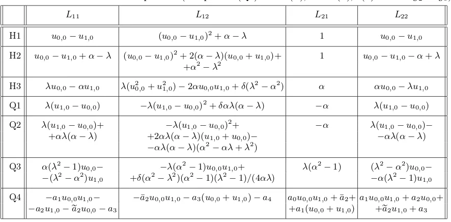
The algorithmic procedure described in [2,9,22] produces a 2×2 matrix Lax pair for the ABS equations, thus ensuring their integrability. It may be written as
Table 1. MatrixLfor the ABS equations (in equation (Q4)a2
=r(α),b2
=r(λ),r(x) = 4x3
−g2x−g3).
L11 L12 L21 L22
H1 u0,0−u1,0 (u0,0−u1,0)2+α−λ 1 u0,0−u1,0 H2 u0,0−u1,0+α−λ (u0,0−u1,0)2+ 2(α−λ)(u0,0+u1,0)+ 1 u0,0−u1,0−α+λ
+α2−λ2
H3 λu0,0−αu1,0 λ(u20,0+u21,0)−2αu0,0u1,0+δ(λ2−α2) α αu0,0−λu1,0
Q1 λ(u1,0−u0,0) −λ(u1,0−u0,0)2+δαλ(α−λ) −α λ(u1,0−u0,0)
Q2 λ(u1,0−u0,0)+ −λ(u1,0−u0,0)2+ −α λ(u1,0−u0,0)− +αλ(α−λ) +2αλ(α−λ)(u1,0+u0,0)− −αλ(α−λ)
−αλ(α−λ)(α2−αλ+λ2) Q3 α(λ2
−1)u0,0− −λ(α2−1)u0,0u1,0+ λ(α2−1) (λ2−α2)u0,0− −(λ2−α2)u1,0 +δ(α2−λ2)(α2−1)(λ2−1)/(4αλ) −α(λ2−1)u1,0 Q4 −a1u0,0u1,0− −¯a2u0,0u1,0−a3(u0,0+u1,0)−a4 a0u0,0u1,0+ ¯a2+a1u0,0u1,0+a2u0,0+
−a2u1,0−ea2u0,0−a3 +a1(u0,0+u1,0) +ea2u1,0+a3
where ℓ = ℓ0,0 = ℓ(u0,0, u1,0;α, λ), t = t0,0 = t(u0,0, u0,1;β, λ), Lij = Lij(u0,0, u1,0;α, λ) and
Mij = Mij(u0,0, u0,1;β, λ), i, j = 1,2. The matrix M can be obtained from L by replacing α withβ and shifting along direction 2 instead of 1. In Table1we give the entries of the matrixL
for the ABS equations.
Note that ℓ and t are computed by requiring that the compatibility condition between L
and M produces the ABS equations (H1)–(H3) and (Q1)–(Q4). The factorℓ can be written as
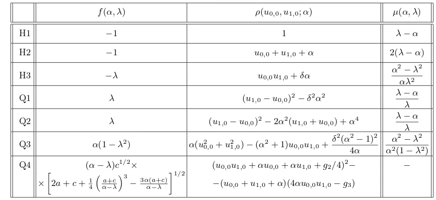
ℓ0,0 =f(α, λ)[ρ(u0,0, u1,0;α)]1/2, (4)
where the functionsf =f(α, λ) is an arbitrary normalization factor. The functionsf =f(α, λ) and ρ = ρ0,0 = ρ(u0,0, u1,0;α) for equations (H1)–(H3) and (Q1)–(Q4) are given in Table 2. A formula similar to (4) holds also for the factor t.
The scalar Lax pairs for the ABS equations may be immediately computed from equation (3). Let us write the scalar equation just for the second componentφof the vector Ψ (the use of the first component would give similar results). For equations (H1)–(H3) and (Q1)–(Q3) it reads
(ρ1,0)1/2φ2,0−(u2,0−u0,0)φ1,0+ (ρ0,0)1/2µφ0,0 = 0, (5)
where the explicit expressions of µ = µ(α, λ) are given in Table 2. The corresponding scalar equation for equation (Q4) takes a different form and needs a separate analysis which will be done in a separate work.
3
Miura transformations for equations (H1)–(H3)
and (Q1)–(Q3)
The aim of this Section is to show the existence of a Miura transformation mapping the scalar spectral problem (5) of equations (H1)–(H3) and (Q1)–(Q3) into the discrete Schr¨odinger spec-tral problem associated with the Volterra lattice [10]
φ−1,0+v0,0φ1,0 =p(λ)φ0,0, (6)
Table 2. Scalar spectral problems for the ABS equations (in equation (Q4) c2 equation (5) is mapped into the scalar spectral problem (6) with
v0,0 =
ρ0,0
(u1,0−u−1,0)(u2,0−u0,0)
, p(λ) = [µ(α, λ)]−1/2. (8)
From these results there follow some remarkable consequences: (i) There exists a Miura trans-formation between all equations of the set (H1)–(H3) and (Q1)–(Q3). Some results on this claim can be found in [7]; (ii) The Miura transformation (8) can be inverted by solving a linear difference equation. Therefore we can in principle use these remarks to find explicit solutions of the ABS equations in terms of the solutions of the Volterra equation.
The following statement holds.
Proof . From equation (8) we get
v0,0(u2,0−u0,0) =
ρ0,0
u1,0−u−1,0
, v−1,0(u0,0−u−2,0) =
ρ−1,0
u1,0−u−1,0
.
Subtracting these relations and taking into account that (see equation (A.11) in [28])
∂u1,0ρ0,0+∂u−1,0ρ−1,0 = 2
ρ0,0−ρ−1,0
u1,0−u−1,0
,
one arrives at
v0,0(u2,0−u0,0)−v−1,0(u0,0−u−2,0) = 1
2 ∂u1,0ρ0,0+∂u−1,0ρ−1,0
. (15)
Writing equation (15) explicitly for equations (H1)–(H3) and (Q1)–(Q3) we obtain
equa-tions (9)–(14).
4
Generalized symmetries of the ABS equations
Lie symmetries of equation (2) are given by those continuous transformations which leave the equation invariant. We refer to [19,31] for a review on symmetries of discrete equations.
From the infinitesimal point of view, Lie symmetries are obtained by requiring the infinite-simal invariant condition
prXb0,0
EE=0 = 0, (16)
where b
X0,0=F0,0(u0,0, u1,0, u0,1, . . .)∂u0,0. (17)
By prXb0,0 we mean the prolongation of the infinitesimal generatorXb0,0 to all points appearing inE = 0.
If F0,0 = F0,0(u0,0) then we get point symmetries and the procedure to construct them from equation (16) is purely algorithmic [19]. If F0,0 = F0,0(u0,0, u1,0, u0,1, . . .) the obtained symmetries are called generalized symmetries. In the case of nonlinear discrete equations, the Lie point symmetries are not very common, but, if the equation is integrable, it is possible to construct an infinite family of generalized symmetries.
In correspondence with the infinitesimal generator (17) we can in principle construct a group transformation by integrating the initial boundary problem
du0,0(ε)
dε =F0,0(u0,0(ε), u1,0(ε), u0,1(ε), . . .), (18)
withu0,0(ε= 0) =v0,0, whereε∈Ris the continuous Lie group parameter andv0,0is a solution of equation (2). This can be done effectively only in the case of point symmetries as in the generalized case we have a nonlinear differential-difference equation for which we cannot find the general solution , but, at most, we can construct particular solutions.
Equation (16) is equivalent to the request that theε-derivative of the equationE = 0, written for u0,0(ε), is identically satisfied on its solutions when the ε-evolution of u0,0(ε) is given by equation (18). This is also equivalent to say that the flows (in the group parameter space) given by equation (18) are compatible or commute withE = 0.
4.1 The ABS equations as B¨acklund transformations of the YdKN equation
In the following we show that the ABS equations may be seen as B¨acklund transformations of the YdKN equation. Moreover we prove that the symmetries of the ABS equations [24,28] are subcases of the YdKN equation. For the sake of clarity we consider in a more detailed way just the case of equation (H3). Similar results can be obtained for the whole ABS list (see Proposition2).
According to [24,28] equation (H3) admits the compatible three-point generalized symmetries
du0,0
dε =
u0,0(u1,0+u−1,0) + 2αδ
u1,0−u−1,0
, (19)
du0,0
dε =
u0,0(u0,1+u0,−1) + 2βδ
u0,1−u0,−1 . (20)
Notice that under the discrete mapn↔m,α↔β, equation (19) goes into equation (20), while equation (H3) is left invariant.
The compatibility between equation (H3) and equation (19) generates a B¨acklund transfor-mation (see an explanation below) of any solution u0,0 of equation (19) into its new solution
e
u0,0 =u0,1, ue1,0 =u1,1. (21)
Thus equation (H3) can be rewritten as a B¨acklund transformation for the differential-difference equation (19)
α(u0,0u1,0+eu0,0ue1,0)−β(u0,0eu0,0+u1,0ue1,0) +δ(α2−β2) = 0. (22)
Moreover, the discrete symmetry n ↔ m, α ↔ β implies the existence of the B¨acklund trans-formation for equation (20)
b
u0,0 =u1,0, bu0,1 =u1,1.
This interpretation of lattice equations as B¨acklund transformations has been discussed for the first time in the differential-difference case in [16]. Examples of B¨acklund transformations similar to equation (22) for Volterra-type equations can be found in [29,11].
In [24, 28] generalized symmetries have been obtained for autonomous ABS equations, i.e. such thatα,β are constants. We present here some results on the non-autonomous case whenα
and β depend onnand m. Similar results can be found in [24].
Let the lattice parameters in equation (2) be such that α is a constant and β = β0 = βm.
Let us consider the following two forms of equation (2)
u1,1 =ξ(u0,0, u1,0, u0,1;α, β0), u0,1 =ζ(u0,0, u1,0, u1,1;α, β0), (23)
and a symmetry
du0,0
dε =f0,0 =f(u1,0, u0,0, u−1,0;α), (24)
given by equation (19). We suppose thatuk,l depends on εin all equations and write down the compatibility condition between equation (23) and equation (24)
f1,1 =f0,0∂u0,0ξ+f1,0∂u1,0ξ+f0,1∂u0,1ξ. (25)
autonomous ABS equations, the compatibility condition (25) is satisfied identically for all values of these variables and of the constant parameterβ. In the non-autonomous case, equation (25) depends only on β0 and α. Therefore the compatibility condition is satisfied also for any m.
So, equation (19) is compatible with equation (H3) also in the case when α is constant, but
β = βm. In a similar way, one can prove that equation (20) is the generalized symmetry of
equation (H3) if β is constant, butα=αn.
Let us now discuss the interpretation of the ABS equations as B¨acklund transformations. Let u0,0 be a solution of equation (24), and the function eu0,0 =eun,m(ε) given by equation (21)
be a solution of equation (23), which is compatible with equation (24). equation (23) can be rewritten as the ordinary difference equation
e
u1,0 =ξ(u0,0, u1,0,eu0,0;α, β0), (26)
whereα is constant,β0 =βm,mis fixed,n∈Z. Differentiating equation (26) with respect toε
and using equation (24) together with the compatibility condition (25), one gets
due1,0
dε −
due0,0
dε ∂eu0,0ξ=f0,0∂u0,0ξ+f1,0∂u1,0ξ =fe1,0−fe0,0∂eu0,0ξ, where
e
fk,0=f(euk+1,0,uek,0,uek−1,0;α) =fk,1, uek,0 =uk,1.
The resulting equation is expressed in the form
Ξ1,0 = Ξ0,0∂ue0,0ξ, Ξk,0 =
duek,0
dε −fek,0. (27)
There is for the ABS equations a formal condition∂eu0,0ξ=∂u0,1ξ6= 0. We suppose here that, for the functions u0,0, ue0,0 under consideration, ∂eu0,0ξ 6= 0 for all n ∈ Z. The function eu0,0 is defined by equation (26) up to an integration functionµ0 =µm(ε). We require thatµ0 satisfies the first order ordinary differential equation given by Ξ0,0|n=0= 0. Then equation (27) implies that Ξ0,0= 0 for all n, i.e.ue0,0 is a solution of equation (24).
So, we start with a solution of a generalized symmetry of the form (24), define a functionue0,0 by the difference equation (26) which is a form of corresponding ABS equation, then we specify the integration function µ0 by the ordinary differential equation Ξ0,0|n=0 = 0, and thus obtain a new solution of equation (24). This solution depends on an integration constant ν0 = νm
and the parameter β0. We can construct in this way the solutions u0,2, u0,3, . . . , u0,N, and the
last of them will depend on 2N arbitrary constants ν0, β0, ν1, β1, . . . , νN−1, βN−1. Using such B¨acklund transformation and starting with a simple initial solution, one can obtain, in principle, a multi-soliton solution. See [6,8] for the construction of some examples of solutions.
The symmetries (19), (20) are Volterra-type equations, namely
du0
dε =f(u1, u0, u−1), (28)
where we have dropped one of the independent indexes n or m, since it does not vary. The Volterra equation corresponds tof(u1, u0, u−1) =u0(u1−u−1). An exhaustive list of differential-difference integrable equations of the form (28) has been obtained in [30] (details can be found in [31]). All three-point generalized symmetries of the ABS equations, with no explicit depen-dence on n,m, have the same structure as equation (19) (see details in Section 4.4below) and are particular cases of the YdKN equation
du0
dε =
R(u1, u0, u−1)
u1−u−1
where
A0 =c1u20+ 2c2u0+c3, B0 =c2u20+c4u0+c5, C0=c3u20+ 2c5u0+c6,
and theci’s are constants. equation (29) has been found by Yamilov in [30], discussed in [21,4],
and in most detailed form in [31]. Its continuous limit goes into the Krichever–Novikov equa-tion [15]. This is the only integrable example of the form (28) which cannot be reduced, in general, to the Toda or Volterra equations by Miura-type transformations. Moreover, equa-tion (29) is also related to the Landau–Lifshitz equation [26]. A generalization of equation (29) with nine arbitrary constant coefficients has been considered in [20].
By a straightforward computation we get the following result: all three-point generalized symmetries in the n-direction with no explicit dependence on n, m for the ABS equations are particular cases of the YdKN equation. For the various equations of the ABS classification the coefficients ci, 1≤i≤6, read
H1 : c1= 0, c2 = 0, c3 = 0, c4 = 0, c5 = 0, c6 = 1, H2 : c1= 0, c2 = 0, c3 = 0, c4 = 0, c5 = 1, c6 = 2α,
H3 : c1= 0, c2 = 0, c3 = 0, c4 = 1, c5 = 0, c6 = 2αδ, Q1 : c1= 0, c2 = 0, c3 =−1, c4 = 1, c5 = 0, c6 =α2δ2, Q2 : c1= 0, c2 = 0, c3 = 1, c4 =−1, c5 =−α2, c6 =α4,
Q3 : c1= 0, c2 = 0, c3 =−4α2, c4 = 2α(α2+ 1), c5 = 0, c6 =−(α2−1)2δ2, Q4 : c1= 1, c2 =−α, c3 =α2, c4 = g42 −α2, c5 = αg42+g23, c6= g
2 2
16+αg3.
Proposition 2. The ABS equations (H1)–(H3) and (Q1)–(Q4) correspond to B¨acklund trans-formations of the particular cases of the YdKN equation (29) listed above. The same holds for the non-autonomous ABS equations, such that α is constant and β = βm or α = αn and β
is constant. Equation (29) and the replacement ui → ui,0 provide the three-point generalized symmetries in the n-direction of the ABS equations with a constantα andβ =βm, while
equa-tion (29) and the replacement ui → u0,i, α → β provide symmetries in the m-direction for the
case α=αn and a constant β.
The non-autonomous case is briefly discussed in [24] where they state that ifαis not constant, then the ABS equations have no local three-point symmetries in then-direction. We shall present three-, five- and many-point generalized symmetries in the m-direction for such equations in Subsection 4.3.
A relation between the ABS equations and differential-difference equations is discussed in [2,5]. In [2] most of the ABS equations are interpreted as nonlinear superposition principles for differential-difference equations of the form
(∂xun+1) (∂xun) =h(un+1, un;α), (30)
wherehis a polynomial ofun+1,un. Equations of the form (30) define B¨acklund transformations
for subcases of the Krichever–Novikov equation
∂tu=∂xxxu−3
2
(∂xxu)2−P(u)
∂xu
, (31)
where P is a fourth degree polynomial with arbitrary constant coefficients. In the case of equations (H1) and (H3) with δ = 0, the corresponding differential-difference equations have a different form, and the resulting KdV-type equations differ from equation (31).
4.2 Miura transformations revised
It is possible to revise the Miura transformations constructed in Section3from the point of view of the generalized symmetries. of the Volterra equation. This is exactly the same Miura transformation we have already pre-sented in Section 3. So, also at the level of the generalized symmetries, we may see that there is a deep relation between equations (H1)–(H3) and (Q1)–(Q3) and the Volterra equation. If equa-tion (29) cannot be transformed to the case with c1 =c2 = 0, using a M¨obius transformation, then it cannot be mapped into the Volterra equation by eu0 = G(u0, u1, u−1, u2, u−2, . . .) [31]. Equation (Q4) is of this kind and thus is the only equation of the ABS list which cannot be related to the Volterra equation.
4.3 Master symmetries
Generalized symmetries of equation (29) will also be compatible with the ABS equations, which are, according to Proposition 2, their B¨acklund transformations. Such symmetries can be con-structed, using the master symmetry of equation (29) presented in [4].
Let us rewrite equation (29) by using the equivalentn-dependent notation (see equation (1)), namely
where ε0 is the continuous symmetry parameter (previously denoted withε). We shall denote with εi,i≥1, the parameters corresponding to higher generalized symmetries
dun
The master symmetry of equation (33) is given by
gn=nfn(0). (35)
According to a general procedure described in [31] we need to introduce an explicit dependence on the parameter τ into the master symmetry (35) and into equation (33) itself. Let the coefficientsci, appearing in the polynomialsAn,Bn,Cn, be functions of τ. Thisτ-dependence
implies thatrn satisfies the following partial differential equation
2∂τrn=rn∂un∂un−1rn−(∂unrn) ∂un−1rn
. (36)
On the left hand side of the above equation, we differentiate only the coefficients of rn with
respect to τ. The right hand side has the same form as rn, but with different coefficients.
Collecting the coefficients of the terms uinujn−1 for various powersi and j, we obtain a system of six ordinary differential equations for the six coefficients ci(τ), whose initial conditions are
ci(0) = ci. Generalized symmetries constructed by using equation (34) explicitly depend on τ.
They remain generalized symmetries for any value of τ, as τ is just a parameter for them and for equation (33). So, going over to the initial conditions, we get generalized symmetries of equation (33) and of the corresponding ABS equations.
Let us derive, as an illustrative example, a formula for the symmetryfn(1)from equation (34).
From equations (33)–(35) it follows that
fn(1)=∂τfn(0)+f
From equation (37) we get the first generalized symmetry
dun
Up to our knowledge this formula is new. It provides five-point generalized symmetries in both n- and m-directions for the ABS equations. Examples of such five-point symmetries for equations (H1) and (Q1) withδ = 0 can be found in [24,27].
Let us clarify the construction of the symmetryfn(1) for equations (H1)–(H3). In these cases
the function rn takes the form
rn= 2c4(τ)unun−1+ 2c5(τ)(un+un−1) +c6(τ),
and equation (36) is equivalent to the system
The initial conditions of system (39) are (see the list above Proposition2)
H1 : c4(0) = 0, c5(0) = 0, c6(0) = 1,
H2 : c4(0) = 0, c5(0) = 1, c6(0) = 2α, H3 : c4(0) = 1, c5(0) = 0, c6(0) = 2αδ,
and its solutions are given by
H1 : c4(τ) = 0, c5(τ) = 0, c6(τ) = 1,
H2 : c4(τ) = 0, c5(τ) = 1, c6(τ) = 2(α−τ),
H3 : c4(τ) = 1, c5(τ) = 0, c6(τ) = 2αδeτ.
Note that the master symmetry with the aboveci(τ) generates τ-dependent symmetries for
aτ-dependent equation, but by fixingτ we obtainτ-independent symmetries for aτ-independent equation. Let us remark that the τ-dependence is independent of the order of the symmetry and it may be used for the construction of all higher symmetries.
So, according to formula (38), we may construct the generalized symmetryfn(1), in the case
of the list H, from the following expressions
H1 : fn(0)= 1
un+1−un−1
, rn= 1, Rn= 0,
H2 : fn(0)= un+1+un−1+ 2(un+α)
un+1−un−1
, rn= 2(un+un−1+α), Rn=−2,
H3 : fn(0)= un(un+1+un−1) + 2αδ
un+1−un−1
, rn= 2(unun−1+αδ), Rn= 2αδ.
It is possible to verify that the symmetries (38) with fn(0), rn, Rn given above are compatible
with both equations (33) and (H1)–(H3).
By using the master symmetry constructed above we can construct infinite hierarchies of many-point generalized symmetries of the ABS equations in both directions. In the non-autonomous cases (see Proposition 2) we provide one hierarchy in the n- or m-direction. The master symmetry and formula (38) will also be useful in the case of the generalizations of the ABS equations presented in the next Subsection. It should be remarked that in [24] the authors constructed master symmetries for all autonomous and non-autonomous ABS equations, which are of a different kind with respect to the ones presented here.
4.4 Generalizations of the ABS equations
Here we discuss the generalization of the ABS equations introduced by Tongas, Tsoubelis and Xenitidis (TTX) in [28]. The TTX equations are autonomous lattice equations of the form (2) which possess only two of the four main properties of the ABS equations: they are affine linear and possess the symmetries of the square.
In terms of the polynomialE, see equation (2), one generates the following function h
h(u0,0, u1,0;α, β) =E∂u0,1∂u1,1E − ∂u0,1E
∂u1,1E
,
which is a biquadratic and symmetric polynomial in its first two arguments. It has been proved in [28] that the TTX equations admit three-point generalized symmetries in then-direction of the form
du0,0
dε =
h u1,0−u−1,0
−1
Of course, there is a similar symmetry in the m-direction. Comparing equations (29), (32) and (40), we see that the symmetry (40) is nothing but the YdKN equation in its general form. This shows that all TTX equations can also be considered as B¨acklund transformations for the YdKN equation. However, they probably describe the general picture for B¨acklund trans-formations of the YdKN equation, which have the form (2). The general formula (38) and the master symmetry discussed in the previous Subsection, provide five- and many-point generalized symmetries of the TTX equations in both directions, thus confirming their integrability.
5
Concluding remarks
In this paper we have considered some further properties of the ABS equations. In particular we have shown that equations (H1)–(H3) and (Q1)–(Q3) can be transformed into equations as-sociated with the spectral problem of the Volterra equation. Therefore all known results for the solution of the Volterra equation can be used to construct solutions of the ABS equations. More-over, all equations of the ABS list, except equation (Q4), can be transformed among themselves by Miura transformations.
The situation of equation (Q4) is somehow different. It is shown that this equation can be thought as a B¨acklund transformation for a subcase of the Yamilov discretization of the Krichever–Novikov equation. But it cannot be related by a Miura transformation to a Volterra-type equation and this explains the complicate form of its scalar spectral problem. The master symmetry constructed for the YdKN equation can, however, be used also in this case to construct generalized symmetries.
It turns out that a generalizations of the ABS equations introduced by Tongas, Tsoubelis and Xenitidis are B¨acklund transformations for the YdKN equation.
Further generalizations of the TTX and ABS equations can be probably obtained by a proper explicit dependence on the point of the lattice not only in the lattice parameters α and β, but also in the Z2-lattice equation itself. The existence of an n-dependent generalization of the YdKN equation, introduced in [20], could help in solving this problem. Such a generalization is integrable in the sense that it has a master symmetry [4] similar to the one presented here.
Acknowledgments
DL, MP and CS have been partially supported by PRIN Project Metodi geometrici nella teoria delle onde non lineari ed applicazioni-2006 of the Italian Minister for Education and Scientific Research. RY has been partially supported by the Russian Foundation for Basic Research (Grant numbers 07-01-00081-a and 06-01-92051-KE-a) and he thanks the University of Roma Tre for hospitality. This work has been done in the framework of the Project Classification of integrable discrete and continuous modelsfinanced by a joint grant from EINSTEIN consortium and RFBR.
References
[1] Adler V.E., On the structure of the B¨acklund transformations for the relativistic lattices,J. Nonlinear Math. Phys.7(2000), 34–56,nlin.SI/0001072.
[2] Adler V.E., Bobenko A.I., Suris Yu.B., Classification of integrable equations on quad-graphs. The consis-tency approach,Comm. Math. Phys.233(2003), 513–543,nlin.SI/0202024.
[3] Adler V.E., Bobenko A.I., Suris Yu.B., Discrete nonlinear hyperbolic equations. Classification of integrable cases,arXiv:0705.1663.
[5] Adler V.E., Suris Yu.B., Q4: integrable master equation related to an elliptic curve,Int. Math. Res. Not. 2004(2004), no. 47, 2523–2553,nlin.SI/0309030.
[6] Adler V.E., Veselov A.P., Cauchy problem for integrable discrete equations on quad-graph,Acta Appl. Math. 84(2004), 237–262,math-ph/0211054.
[7] Atkinson J., B¨acklund transformations for integrable lattice equations,J. Phys. A: Math. Theor.41(2008) 135202, 8 pages,arXiv:0801.1998.
[8] Atkinson J., Hietarinta J., Nijhoff F.W., Seed and soliton solutions for Adler’s lattice equation,J. Phys. A: Math. Theor.40(2007), F1–F8,nlin.SI/0609044.
[9] Bobenko A.I., Suris Yu.B., Integrable systems on quad-graphs, Int. Math. Res. Not.2002(2002), no. 11, 573–611,nlin.SI/0110004.
[10] Case K.M., Kac M., A discrete version of the inverse scattering problem,J. Math. Phys.14(1973), 594–603. [11] Chiu S.C., Ladik J.F., Generating exactly soluble nonlinear discrete evolution equations by a generalized
Wronskian technique,J. Math. Phys.18(1977), 690–700.
[12] Francoise J.P., Naber G., Tsou S.T. (Editors), Encyclopedia of mathematical physics, Elsevier, 2007. [13] Galor O., Discrete dynamical systems, Springer, Berlin, 2007.
[14] Hirota R., Nonlinear partial difference equations. I. A difference analog of the Korteweg–de Vries equation, J. Phys. Soc. Japan43(1977), 1423–1433.
Hirota R., Nonlinear partial difference equations. III. Discrete sine-Gordon equation,J. Phys. Soc. Japan 43(1977), 2079–2086.
[15] Krichever I.M., Novikov S.P., Holomorphic bundles over algebraic curves, and nonlinear equations,Uspekhi Mat. Nauk35(1980), no. 6, 47–68 (in Russian).
[16] Levi D., Nonlinear differential-difference equations as B¨acklund transformations, J. Phys. A: Math. Gen. 14(1981), 1083–1098.
[17] Levi D., Petrera M., Continuous symmetries of the lattice potential KdV equation,J. Phys. A: Math. Theor. 40(2007), 4141–4159,math-ph/0701079.
[18] Levi D., Petrera M., Scimiterna C., The lattice Schwarzian KdV equation and its symmetries,J. Phys. A: Math. Theor.40(2007), 12753–12761,math-ph/0701044.
[19] Levi D., Winternitz P., Continuous symmetries of difference equations,J. Phys. A: Math. Gen.39(2006), R1–R63,nlin.SI/0502004.
[20] Levi D., Yamilov R.I., Conditions for the existence of higher symmetries of evolutionary equations on the lattice,J. Math. Phys.38(1997), 6648–6674.
[21] Mikhailov A.V., Shabat A.B., Yamilov R.I., The symmetry approach to the classification of nonlinear equations. Complete lists of integrable systems,Uspekhi Mat. Nauk42(1887), no. 4, 3–53 (English transl.: Russian Math. Surveys42(1987), no. 4, 1–63).
[22] Nijhoff F.W., Lax pair for the Adler (lattice Krichever–Novikov) system,Phys. Lett. A297(2002), 49–58,
nlin.SI/0110027.
[23] Nijhoff F.W., Capel H.W., The discrete Korteweg–de Vries equation,Acta Appl. Math.39(1995), 133–158. [24] Rasin O.G., Hydon P.E., Symmetries of integrable difference equations on the quad-graph, Stud. Appl.
Math.119(2007), 253–269.
[25] Sandevan J.T., Discrete dynamical systems. Theory and applications, The Clarendon Press, Oxford Univer-sity Press, New York, 1990.
[26] Shabat A.B., Yamilov R.I., Symmetries of nonlinear chains, Algebra i Analiz 2 (1990), 183–208 (English transl.: Leningrad Math. J.2(1991), 377–400).
[27] Tongas A., Tsoubelis D., Papageorgiou V., Symmetries and group invariant reductions of integrable partial difference equations, in Proc. 10th Int. Conf. in Modern Group Analysis (October 24–31, 2004, Larnaca, Cyprus), Editors N.H. Ibragimov, C. Sophocleous and P.A. Damianou, 2004, 222–230.
[28] Tongas A., Tsoubelis D., Xenitidis P., Affine linear andD4 symmetric lattice equations: symmetry analysis and reductions,J. Phys. A: Math. Theor.40(2007), 13353–13384,arXiv:0707.3730.
[29] Yamilov R.I., Construction scheme for discrete Miura transformations,J. Phys. A: Math. Gen. 27(1994), 6839–6851.
[30] Yamilov R.I., Classification of discrete evolution equations, Uspekhi Mat. Nauk38(1983), no. 6, 155–156 (in Russian).