Paths of Brownian Motion
Yuval Peres
Lecture notes edited by B´alint Vir´ag, Elchanan Mossel and Yimin Xiao
Version of November 1, 2001
2
Chapter 1. Brownian Motion 1 1. Motivation – Intersection of Brownian paths 1
2. Gaussian random variables 1
3. L´evy’s construction of Brownian motion 4
4. Basic properties of Brownian motion 6
5. Hausdorff dimension and Minkowski dimension 11 6. Hausdorff dimension of the Brownian path and the Brownian graph 13
7. On nowhere differentiability 17
8. Strong Markov property and the reflection principle 18
9. Local extrema of Brownian motion 20
10. Area of planar Brownian motion paths 20
11. Zeros of the Brownian motion 22
12. Harris’ Inequality and its consequences 27 13. Points of increase for random walks and Brownian motion 29 14. Frostman’s Lemma, energy, and dimension doubling 33
15. Skorokhod’s representation 39
16. Donsker’s Invariance Principle 43
17. Harmonic functions and Brownian motion inRd 47 18. Maximum principle for harmonic functions 50
19. The Dirichlet problem 51
20. Polar points and recurrence 52
21. Capacity and harmonic functions 54
22. Kaufman’s theorem on uniform dimension doubling 57
23. Packing dimension 59
24. Hausdorff dimension and random sets 60 25. An extension of L´evy’s modulus of continuity 61
References 63
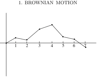
CHAPTER 1
Brownian Motion
1. Motivation – Intersection of Brownian paths
Consider a number of Brownian motion paths started at different points. Say that they intersect if there is a point which lies on all of the paths. Do the paths intersect? The answer to this question depends on the dimension:
• In R2, any finite number of paths intersect with positive probability (this is a theorem of Dvoretsky, Erd˝os, Kakutani in the 1950’s),
• InR3, two paths intersect with positive probability, but not three (this is a theorem of Dvoretsky, Erd˝os, Kakutani and Taylor, 1957),
• In Rd ford≥4, no pair of paths intersect with positive probability.
The principle we will use to establish these results is intersection equivalence between Brownian motion and certain random Cantor-type sets. Here we will introduce the concept for R3 only. Partition the cube [0,1]3 in eight congruent sub-cubes, and keep each of the sub-cubes with probability12. For each cube that remained at the end of this stage, partition it into eight sub-cubes, keeping each of them with probability 12, and so on. Let Q 3,12
denote the limiting set— that is, the intersection of the cubes remaining at all steps. This set is not empty with positive probability, since, if we consider that the remaining sub-cubes of a given cube as its “children” in a branching process, then the expected number of offsprings is four, so this process has positive probability not to die out.
One can prove that, there exist two positive constantsC1, C2 such that, if Λ is a closed subset of [0,1]3, and {Bt} is a Brownian motion started at a point uniformly chosen in [0,1]3, then:
C1P
Q
3,1
2
∩Λ6=∅
≤P(∃t≥0 Bt∈Λ)≤C2P
Q
3,1
2
∩Λ6=∅
The motivation is that, though the intersection of two independent Brownian paths is a complicated object, the intersection of two sets of the formQ 3,12 is a set of the same kind—namely, Q 3,14. The previously described branching process dies out as soon as we intersect more than two of these Cantor-type sets—hence the result about intersection of paths in R3.
2. Gaussian random variables
Brownian motion is at the meeting point of the most important categories of stochastic processes: it is a martingale, a strong Markov process, a process with independent and stationary increments, and a Gaussian process. We will construct Brownian motion as a specific Gaussian process. We start with the definitions of Gaussian random variables:
Definition2.1. A real-valued random variableXon a probability space (Ω,F,P) has a standard Gaussian(orstandard normal) distribution if
P(X > x) = √1 2π
Z +∞
x
e−u2/2du
A vector-valued random variable X has an n-dimensional standard Gaussian dis-tribution if itsncoordinates are standard Gaussian and independent.
A vector-valued random variable Y : Ω → Rp is Gaussian if there exists a vector-valued random variableXhaving an n-dimensional standard Gaussian distribution, ap×n
matrixA and ap-dimensional vectorb such that:
Y =AX+b (2.1)
We are now ready to define the Gaussian processes.
Definition 2.2. A stochastic process (Xt)t∈I is said to be a Gaussian processif for allkand t1, . . . , tk∈I the vector (Xt1, . . . , Xtk)
t is Gaussian.
Recall that the covariance matrix of a random vector is defined as
Cov(Y) =E(Y −EY)(Y −EY)t
Then, by the linearity of expectation, the Gaussian vectorY in (2.1) has Cov(Y) =AAt.
Recall that ann×nmatrixAis said to be orthogonalifAAt=I
n. The following lemma shows that the distribution of a Gaussian vector is determined by its mean and covariance.
Lemma 2.3.
(i) IfΘ is an orthogonal n×n matrix and X is an n-dimensional standard Gaussian vector, then ΘX is also an n-dimensional standard Gaussian vector.
(ii)IfY andZ are Gaussian vectors in Rn such that EY =EZ andCov(Y) = Cov(Z), then Y and Z have the same distribution.
Proof.
(i) As the coordinates of X are independent standard Gaussian, X has density given by:
f(x) = (2π)−n2e−kxk2/2
where k · k denotes the Euclidean norm. Since Θ preserves this norm, the density of X is invariant under Θ.
(ii) It is sufficient to consider the case when EY =EZ = 0. Then, using Definition 2.1, there exist standard Gaussian vectorsX1,X2 and matricesA, C so that
Y =AX1 and Z =CX2.
By adding some columns of zeroes toA or C if necessary, we can assume that X1, X2 are both k-vectors for somekand A,C are bothn×k matrices.
2. GAUSSIAN RANDOM VARIABLES 3
form a basis for the space A. For any matrixM let Mi denote the ith row vector of M, and define the linear map Θ fromA toC by
AiΘ =Ci fori= 1, . . . , ℓ.
We want to check that Θ is an isomorphism. Assume that there is a vectorv1A1+· · ·+vℓAℓ whose image is 0. Then the k-vector v = (v1, v2, . . ., vℓ,0, . . .,0) satisfies vtC = 0, and so kvtAk2 = vtAAtv = vtCCtv = 0, giving vtA = 0. This shows that Θ is one-to-one, in particular dimA ≤ dimC. By symmetry A and C must have the same dimension, so Θ is an isomorphism.
As the coefficient (i, j) of the matrixAAtis the scalar product ofAi andAj, the identity
AAt =CCt implies that Θ is an orthogonal transformation from A to C. We can extend it to map the orthocomplement ofA to the orthocomplement ofCorthogonally, getting an orthogonal map Θ :Rk→ Rk. Then
Y =AX1, Z =CX2=AΘX2, and (ii) follows from (i).
Thus, the first two moments of a Gaussian vector are sufficient to characterize its distri-bution, hence the introduction of the notationN(µ,Σ) to designate the normal distribution with expectationµ and covariance matrix Σ. A useful corollary of this lemma is:
Corollary 2.4. Let Z1, Z2 be independent N(0, σ2) random variables. Then Z1+Z2 andZ1−Z2 are two independent random variables having the same distribution N(0,2σ2).
Proof. σ−1(Z
1, Z2) is a standard Gaussian vector, and so, if: Θ = √1
2
1 1 1 −1
then Θ is an orthogonal matrix such that
(√2σ)−1(Z1+Z2, Z1−Z2)t= Θσ−1(Z1, Z2)t, and our claim follows from part (i)of the Lemma.
As a conclusion of this section, we state the following tail estimate for the standard Gaussian distribution:
Lemma 2.5. Let Z be distributed as N(0,1). Then for all x≥0: x
x2+ 1 1 √
2πe
−x2/2
≤P(Z > x)≤ 1 x
1 √
2πe
−x2/2
Proof. The right inequality is obtained by the estimate:
P(Z > x)≤
Z +∞
x
u x
1 √
2πe
−u2/2
du
since, in the integral,u≥x. The left inequality is proved as follows: Let us define
f(x) :=xe−x2/2−(x2+ 1)
Z +∞
x
We remark that f(0)<0 and limx→+∞f(x) = 0.Moreover,
f′(x) = (1−x2+x2+ 1)e−x2/2−2x Z +∞
x
e−u2/2du
= −2x
Z +∞
x
e−u2/2du− 1 xe
−x2/2
,
so the right inequality implies f′(x) ≥0 for all x ≥0. This implies f(x) ≤0, proving the lemma.
3. L´evy’s construction of Brownian motion
3.1. Definition. Standard Brownian motion on an intervalI = [0, a] or I = [0,∞) is defined by the following properties:
Definition 3.1. A real-valued stochastic process {Bt}t∈I is a standard Brownian
motionif it is a Gaussian process such that: (i) B0 = 0,
(ii) ∀k natural and∀t1 < . . . < tk inI: Btk−Btk−1, . . . , Bt2−Bt1 are independent, (iii) ∀t, s∈I witht < s Bs−Bt has N(0, s−t) distribution.
(iv) Almost surely,t7→Bt is continuous onI.
As a corollary of this definition, one can already remark that for allt, s∈I: Cov(Bt, Bs) =s∧t.
Indeed, assume that t ≥ s. Then Cov(Bt, Bs) = Cov(Bt− Bs, Bs) + Cov(Bs, Bs) by bilinearity of the covariance. The first term vanishes by the independence of increments, and the second term equalssby properties (iii) and (i). Thus by Lemma 2.3 we may replace properties (ii) and (iii) in the definition by:
• For all t, s∈I, Cov(Bt, Bs) =t∧s. • For all t∈I,Bt hasN(0, t) distribution. or by:
• For all t, s∈I witht < s,Bt−Bs andBs are independent. • For all t∈I,Bt hasN(0, t) distribution.
Kolmogorov’s extension theorem implies the existence of any countable time set sto-chastic process{Xt}if we know its finite-dimensional distributions and they are consistent. Thus, standard Brownian motion could be easily constructed on any countable time set. However knowing finite dimensional distributions is not sufficient to getcontinuous paths, as the following example shows.
Example 3.2. Suppose that standard Brownian motion {Bt} on [0,1] has been con-structed, and consider an independent random variable U uniformly distributed on [0,1]. Define:
˜
Bt=
Bt ift6=U 0 otherwise
3. L´EVY’S CONSTRUCTION OF BROWNIAN MOTION 5
In measure theory, one often identifies functions with their equivalence class for almost-everywhere equality. As the above example shows, it is important not to make this iden-tification in the study of continuous-time stochastic processes. Here we want to define a probability measure on the set of continuous functions.
3.2. Construction. The following construction, due to Paul L´evy, consist of choosing the “right” values for the Brownian motion at each dyadic point of [0,1] and then inter-polating linearly between these values. This construction is inductive, and, at each step, a process is constructed, that has continuous paths. Brownian motion is then the uniform limit of these processes—hence its continuity. We will use the following basic lemma. The proof can be found, for instance, in Durrett (1995).
Lemma 3.3 (Borel-Cantelli). Let{Ai}i=0,...,∞ be a sequence of events, and let
{Ai i.o.}= lim sup i→∞
Ai = ∞
\
i=0 ∞
[
j=i
Aj,
where “i.o.” abbreviates “infinitely often”.
(i)IfP∞i=0P(Ai)<∞, then P(Aii.o.) = 0.
(ii) If{Ai} are pairwise independent, andP∞i=0P(Ai) =∞, thenP(Aii.o.) = 1. Theorem 3.4 (Wiener 1923). Standard Brownian motion on [0,∞) exists.
Proof. (L´evy 1948)
We first construct standard Brownian motion on [0,1]. Forn≥0, letDn={k/2n: 0≤
k≤ 2n}, and let D =SDn. Let {Zd}d∈D be a collection of independent N(0,1) random variables. We will first construct the values of B on D. Set B0 = 0, and B1 = Z1. In an inductive construction, for eachnwe will constructBd for alld∈Dnso that
(i) For allr < s < tinDn, the increment Bt−Bs has N(0, t−s) distribution and is independent ofBs−Br.
(ii) Bd ford∈Dn are globally independent of theZd ford∈D\Dn.
These assertions hold for n = 0. Suppose that they hold for n−1. Define, for all
d∈Dn\Dn−1, a random variableBd by
Bd=
Bd−+Bd+
2 +
Zd
2(n+1)/2 (3.1) where d+ = d+ 2−n, and d− = d−2−n, and both are in Dn−1. Since 12[Bd+ −Bd−] is
N(0,1/2n+1) by induction, andZ
d/2(n+1)/2 is an independentN(0,1/2n+1), their sum and their difference,Bd−Bd− andBd+−Bdare bothN(0,1/2n) and independent by Corollary 2.4. Assertion (i) follows from this and the inductive hypothesis, and (ii) is clear.
Having thus chosen the values of the process onD, we now “interpolate” between them. Formally, let F0(x) =xZ1, and forn≥1, let let us introduce the function:
Fn(x) =
2−(n+1)/2Zx forx∈Dn\Dn−1, 0 forx∈Dn−1,
linear between consecutive points inDn.
These functions are continuous on [0,1], and for allnand d∈Dn
Bd= n
X
i=0
Fi(d) = ∞
X
i=0
Fi(d). (3.3)
This can be seen by induction. Suppose that it holds forn−1. Letd∈Dn−Dn−1. Since for 0≤i≤n−1 Fi is linear on [d−, d+], we get
n−1
X
i=0
Fi(d) = n−1
X
i=1
Fi(d−) +Fi(d+)
2 =
Bd−+Bd+
2 . (3.4)
Since Fn(d) = 2−(n+1)/2Zd, comparing (3.1) and (3.4) gives (3.3). On the other hand, we have, by definition ofZd and by Lemma 2.5:
P |Zd| ≥c√n≤exp
−c 2n 2
for n large enough, so the series P∞n=0Pd∈DnP(|Zd| ≥ c√n) converges as soon as c > √
2 log 2. Fix such a c. By the Borel-Cantelli Lemma 3.3 we conclude that there exists a random but finiteN so that for all n > N and d∈Dnwe have|Zd|< c√n, and so:
kFnk∞< c√n2−n/2. (3.5)
This upper bound implies that the series P∞n=0Fn(t) is uniformly convergent on [0,1], and so it has a continuous limit, which we call {Bt}. All we have to check is that the increments of this process have the right finite-dimensional joint distributions. This is a direct consequence of the density of the setD in [0,1] and the continuity of paths. Indeed, let t1 > t2 > t3 be in [0,1], then they are limits of sequences t1,n, t2,n and t3,n in D, respectively. Now
Bt3 −Bt2 = lim
k→∞(Bt3,k −Bt2,k)
is a limit of Gaussian random variables, so itself is Gaussian with mean 0 and vari-ance limn→∞(t3,n−t2,n) = t3 −t2. The same holds for Bt2 −Bt1, moreover, these two random variables are limit of independent random variables, since for n large enough,
t1,n > t2,n > t3,n. Applying this argument for any number of increments, we get that {Bt}has independent increments such that and for alls < tin [0,1]Bt−Bs hasN(0, t−s) distribution.
We have thus constructed Brownian motion on [0,1]. To conclude, if {Btn}t for n≥0 are independent Brownian motions on [0,1], then
Bt=Bt⌊−⌊t⌋t⌋+
X
0≤i<⌊t⌋
B1i
meets our definition of Brownian motion on [0,∞).
4. Basic properties of Brownian motion
Let {B(t)}t≥0 be a standard Brownian motion, and let a6= 0. The following scaling
relation is a simple consequence of the definitions. {1
4. BASIC PROPERTIES OF BROWNIAN MOTION 7
Also, define the time inversionof {Bt}as
W(t) =
0 t= 0;
tB(1t) t >0. We claim thatW is a standard Brownian motion. Indeed,
Cov(W(t), W(s)) =tsCov(B(1
t,
1
s)) =ts(
1
t ∧
1
s) =t∧s,
so W and B have the same finite dimensional distributions, and they have the same dis-tributions as processes on the rational numbers. Since the paths of W(t) are continuous except maybe at 0, we have
lim
t↓0W(t) = limt↓0,t∈QW(t) = 0 a.s.
so the paths of W(t) are continuous on [0,∞) a.s. As a corollary, we get Corollary 4.1. [Law of Large Numbers for Brownian motion]
lim t→∞
B(t)
t = 0 a.s.
Proof. limt→∞ B(tt) = limt→∞W(1t) = 0 a.s.
Exercise 4.2. Prove this result directly. Use the usual Law of Large Numbers to show that limn→∞ B(nn) = 0. Then show that B(t) does not oscillate too much between n and
n+ 1.
Remark. The symmetry inherent in the time inversion property becomes more appar-ent if one considers the Ornstein-Uhlenbeck diffusion, which is given by
X(t) =e−tB(e2t)
This is a stationary Markov chain with X(t) ∼ N(0,1) for all t. It is a diffusion with a drift toward the origin proportional to the distance from the origin. Unlike Brownian motion, the Ornstein-Uhlenbeck diffusion is time reversible. The time inversion formula gives{X(t)}t≥0 =d {X(−t)}t≥0. For t near−∞,X(t) relates to the Brownian motion near 0, and fortnear ∞,X(t) relates to the Brownian motion near ∞.
One of the advantages of L´evy’s construction of Brownian motion is that it easily yields a modulus of continuity result. Following L´evy, we defined Brownian motion as an infinite sum P∞n=0Fn, where each Fn is a piecewise linear function given in (3.2). Its derivative exists almost everywhere, and by definition and (3.5)
kFn′k∞≤ k
Fnk∞
2−n ≤C1(ω) + √
n2n/2 (4.1)
The random constantC1(ω) is introduced to deal with the finitely many exceptions to (3.5). Now fort, t+h∈[0,1], we have
|B(t+h)−B(t)| ≤X n
|Fn(t+h)−Fn(t)| ≤
X
n≤ℓ
hkFn′k∞+X n>ℓ
By (3.5) and (4.1) if ℓ > N for a randomN, then the above is bounded by
The inequality holds because each series is bounded by a constant times its dominant term. Choosingℓ=⌊log2(1/h)⌋, and choosing C(ω) to take care of the cases whenℓ≤N, we get
|B(t+h)−B(t)| ≤C(ω)
r
hlog2 1
h. (4.3)
The result is a (weak) form of L´evy’s modulus of continuity. This is not enough to make {Bt} a differentiable function since
√
h≫h for smallh. But we still have Corollary 4.3. For every α < 12, Brownian paths areα - H¨older a.s.
Exercise 4.4. Show that a Brownian motion is a.s. not 12 - H¨older.
Remark. There does exist at=t(ω) such that|B(t+h)−B(t)| ≤C(ω)h12 for everyh, a.s. However, suchthave measure 0. This is the slowest movement that is locally possible. Solution. LetAk,n be the event thatB((k+ 1)2−n)−B(k2−n)> c√n2−n/2. Then Lemma 2.5
We remark that the paths are a.s. not 1
2-H¨older. Indeed, the log2(h1) factor in (4.3) cannot be
ignored. We will see later that the Hausdorff dimension of the graph of Brownian motion is 32 a.s.
Having proven that Brownian paths are somewhat “regular”, let us see why they are “bizarre”. One reason is that the paths of Brownian motion have no intervals of mono-tonicity. Indeed, if [a, b] is an interval of monotonicity, then dividing it up into n equal sub-intervals [ai, ai+1] each incrementB(ai)−B(ai+1) has to have the same sign. This has probability 2·2−n, and taking n→ ∞ shows that the probability that [a, b] is an interval of monotonicity must be 0. Taking a countable union gives that there is no interval of monotonicity with rational endpoints, but each monotone interval would have a monotone rational sub-interval.
We will now show that for any timet0, Brownian motion is not differentiable att0. For this, we need a simple proposition.
4. BASIC PROPERTIES OF BROWNIAN MOTION 9
Remark. Comparing this with Corollary 4.1, it is natural to ask what sequence B(n) should be divided by to get a lim sup which is greater than 0 but less than∞. An answer is given by the law of the iterated logarithm in a later section.
The proof of (4.4) relies on the following standard fact, whose proof can be found, for example, in Durrett (1995). Consider a probability measure on the space of real sequences, and letX1, X2, . . . be the sequence of random variables it defines. An event, that is a mea-surable set of sequences,Ais exchangeable ifX1, X2, . . . satisfyAimplies thatXσ1, Xσ2, . . . satisfy A for all finite permutationsσ. Herefinite permutation means that σn =n for all sufficiently largen.
Proposition 4.6 (Hewitt-Savage 0-1 Law). IfA is an exchangeable event for an i.i.d. sequence then P(A) is 0 or 1.
Proof of Proposition 4.5.
P(B(n)> c√n i.o.)≥lim sup
n→∞ P(B(n)> c √
n)
By the scaling property, the expression in the lim sup equalsP(B(1)> c), which is positive. LettingXn=B(n)−B(n−1) the Hewitt-Savage 0-1 law gives thatB(n)> c√ninfinitely often. Taking the intersection over all naturalcgives the first part of (4.4), and the second is proved similarly.
The two claims of Proposition 4.5 together mean thatB(t) crosses 0 for arbitrarily large values of t. If we use time inversionW(t) =tB(1t), we get that Brownian motion crosses 0 for arbitrarily small values of t. Letting ZB = {t : B(t) = 0}, this means that 0 is an accumulation point from the right forZB. But we get even more. For a function f, define the upper and lower right derivatives
D∗f(t) = lim sup h↓0
f(t+h)−f(t)
h ,
D∗f(t) = lim inf h↓0
f(t+h)−f(t)
h .
Then
D∗W(0)≥lim sup n→∞
W(1n)−W(0) 1 n
≥lim sup n→∞
√
n W(n1) = lim supB√(n) n
which is infinite by Proposition 4.5. Similarly, D∗W(0) = −∞, showing that W is not differentiable at 0.
Corollary 4.7. Fix t0 ≥ 0. Brownian motion W a.s. satisfies D∗W(t0) = +∞, D∗W(t0) = −∞, and t0 is an accumulation point from the right for the level set {s : W(s) =W(t0)}.
Proof. t→W(t0+t)−W(t0) is a standard Brownian motion.
t0-s must have Lebesgue measure 0. This is true in general. Suppose A is a measurable event (set of paths) such that
∀t0, P(t→W(t0+t)−W(t0) satisfiesA) = 1.
Let Θt be the operator that shifts paths byt. ThenP(Tt0∈QΘt0(A)) = 1,hereQis the set
of rational numbers. In fact, the Lebesgue measure of points t0 so thatW does not satisfy Θt0(A) is 0 a.s. To see this, apply Fubini to the double integral
Z Z ∞
0
1(W /∈Θt0(A))dt0 dP(W)
Exercise4.8. Show that∀t0, P(t0 is a local maximum for B) = 0,but a.s. local maxima are a countable dense set in (0,∞).
Nowhere differentiability of Brownian motion therefore requires a more careful argument than non-differentiability at a fixed point.
Theorem 4.9 (Paley, Wiener and Zygmund 1933). A.s. Brownian motion is nowhere differentiable. Furthermore, almost surely for allt eitherD∗B(t) = +∞ or D∗B(t) =−∞.
Remark. For local maxima we have D∗B(t) ≤0, and for local minima, D∗B(t) ≥0, so it is important to have the either-or in the statement.
Proof. (Dvoretsky, Erd˝os and Kakutani 1961) Suppose that there is at0 ∈[0,1] such that−∞< D∗B(t0)≤D∗B(t0) <∞. Then for some finite constantM we would have
sup h∈[0,1]
|B(t0+h)−B(t0)|
h ≤M. (4.5)
If t0 is contained in the binary interval [(k−1)/2n, k/2n] for n >2, then for all 1≤j ≤n the triangle inequality gives
|B((k+j)/2n)−B((k+j−1)/2n)| ≤M(2j+ 1)/2n. (4.6) Let Ωn,k be the event that (4.6) holds forj= 1, 2, and 3. Then by the scaling property
P(Ωn,k)≤P
|B(1)| ≤7M/√2n3,
which is at most (7M2−n/2)3, since the normal density is less than 1/2. Hence
P 2n
[
k=1 Ωn,k
!
≤2n(7M2−n/2)3= (7M)32−n/2,
whose sum over allnis finite. By the Borel-Cantelli lemma:
P((4.5) is satisfed)≤P 2n
[
k=1
Ωn,k for infinitely manyn
!
= 0.
That is, for sufficiently large n, there are no three good increments in a row so (4.5) is satisfied.
Exercise4.10. Letα >1/2. Show that a.s. for allt >0,∃h >0 such that|B(t+h)−
5. HAUSDORFF DIMENSION AND MINKOWSKI DIMENSION 11
forn >2, then the triangle inequality gives
|B(k+j
since the normal density is less than 1/2. Hence
P(
5. Hausdorff dimension and Minkowski dimension
Definition5.1 (Hausdorff 1918). LetA be a subset of a metric space. Forα >0, and a possibly infiniteǫ >0 define a measure of size forA by
Hα(ǫ)(A) = inf{
where|·|applied to a set means its diameter. The quantityH(∞)(A) is called theHausdorff contentof A. Define theα-dimensionalHausdorff measureof Aas
Hα(A) = lim value is called the Hausdorff dimension ofA.
Note that given β > α >0 and Hα
(ǫ)(A)<∞, we have Hβ(ǫ)(A)≤ǫ(β−α)Hα(ǫ)(A).
where the inequality follows from the fact that |Aj|β ≤ ǫ(β−α)|Aj|α for a covering set Aj of diameter ≤ ǫ. Since ǫ is arbitrary here, we see that if Hα(A) < ∞, then Hβ(A) = 0.
Therefore, we can also define the Hausdorff dimension of A as
sup{α >0 :Hα(A) =∞}.
Now let us look at another kind of dimension defined as follows.
Definition 5.3. The upper and lower Minkowski dimension (also called“Box” dimension) ofA is defined as
dimM(A) = lim ǫ↓0
logNǫ(A) log(1/ǫ) , dimM(A) = lim
ǫ↓0
logNǫ(A) log(1/ǫ) ,
whereNǫ(A) is the minimum number of balls of radiusǫneeded to coverA. If dimM(A) = dimM(A), we call the common value theMinkowski dimensionofA, denoted by dimM.
Exercise 5.4. Show that dimM([0,1]d) =d.
Proposition 5.5. For any setA, we have dimH(A)≤dimM(A).
Proof. By definition,Hα
(2ǫ)(A)≤Nǫ(A)(2ǫ)α. If α >dimM(A), then we have limǫ↓0Nǫ(A)(2ǫ)α= 0.
It then follows thatHα(A) = 0 and hence dim
H(A)≤dimM(A).
We now look at some examples to illustrate the definitions above. Let A be all the rational numbers in the unit interval. Since for every setDwe have dimM(D) = dimM(D), we get dimM(A) = dimM(A) = dimM([0,1]) = 1. On the other hand, a countable set A
always has dimH(A) = 0. This is because for any α, ǫ > 0, we can cover the countable points inA by balls of radiusǫ/2,ǫ/4,ǫ/8, and so on. Then
Hα
(ǫ)(A)≤
X
j
|Aj|α≤
X
j
(ǫ2−j)α<∞.
Another example is the harmonic sequence A={0}S{1/n}n≥1. It is a countable set, so it has Hausdorff dimension 0. It can be shown that dimM(A) = 1/2. (Those points inAthat are less than√ǫcan be covered by 1/√ǫballs of radiusǫ. The rest can be covered by 2/√ǫ
balls of radiusǫ, one on each point.)
6. HAUSDORFF DIMENSION OF THE BROWNIAN PATH AND THE BROWNIAN GRAPH 13
Proposition 5.6. Letf : [0,1]→R be a β-H¨older continuous function. Then
dimM(Gf)≤2−β.
Proof. Since f is β-H¨older, there exists a constant C1 such that, if |t−s| ≤ ǫ, then |f(t)−f(s)| ≤C1ǫβ =C1ǫ·(1/ǫ1−β). Hence, the minimum number of balls of radius ǫ to coverGf satisfiesNǫ(Gf)≤C2(1/ǫ2−β) for some other constant C2.
Corollary 5.7.
dimH(GB)≤dimM(GB)≤dimM(GB)≤3/2. a.s.
A function f : [0,1]→R is called “reverse” β-H¨older if there exists a constant C > 0 such that for any interval [t, s], there is a subinterval [t1, s1] ⊂ [t, s], such that |f(t1)− f(s1)| ≥C|t−s|β.
Proposition 5.8. Let f : [0,1] → R be β-H¨older and “reverse” β-H¨older. Then
dimM(Gf) = 2−β.
Remark. It follows from the hypotheses of the above proposition that such a function
f has the property dimH(Gf)>1.(Przytycki-Urbansky, 1989.) Exercise 5.9. Prove Proposition 5.8.
Example 5.10. The Weierstrass nowhere differentiable function
W(t) = ∞
X
n=0
ancos(bnt),
ab >1, 0< a <1 is β-H¨older and “reverse”β-H¨older for some 0< β <1. For example, if
a= 1/2,b= 4, thenβ = 1/2.
Lemma 5.11. Suppose X is a complete metric space. Let f :X→ Y be β-H¨older. For any A ⊂ X, we have dimHf(A) ≤ dimH(A)/β. Similar statements for dimM and dimM
are also true.
Proof. If dimH(A)< α <∞, then there exists a cover{Aj}such thatA⊂SjAj and
P
j|Aj|α < ǫ. Then {f(Aj)} is a cover for f(A), and |f(Aj)| ≤ C|Aj|β, where C is the constant from theβ-H¨older condition. Thus,
X
j
|f(Aj)|α/β≤Cα/β
X
j
|Aj|α< Cα/βǫ→0
asǫ→0, and hence dimHf(A)≤α/β.
Corollary 5.12. ForA⊂[0,∞), we have dimHB(A)≤2 dimH(A)∧1 a.s.
6. Hausdorff dimension of the Brownian path and the Brownian graph
Define thed-dimensional standard Brownian motion whose coordinates are independent one dimensional standard Brownian motions. Its distribution is invariant under orthogonal transformations of Rd, since Gaussian random variables are invariant to such transforma-tions by Lemma 2.3. Ford≥2 it is interesting to look at the image set of Brownian motion. We will see that planar Brownian motion is neighborhood recurrent, that is, it visits every neighborhood in the plane infinitely often. In this sense, the image of planar Brownian motion is comparable to the plane itself; another sense in which this happens is that of Hausdorff dimension: the image of planar and higher dimensional Brownian motion has Hausdorff dimension two. Summing up, we will prove
Theorem 6.1 (Taylor 1953). Let B be d−dimensional Brownian motion defined on the time set [0,1]. Then
dimHGB = 3/2 a.s.
Moreover, if d≥2, then
dimHB[0,1] = 2 a.s.
Higher dimensional Brownian motion therefore doubles the dimension of the time line. Naturally, the question arises whether this holds for subsets of the time line as well. In certain sense, this even holds ford= 1: note the “∧d” in the following theorem.
Theorem 6.2 (McKean 1955). For every subset A of [0,∞), the image of A under d dimensional Brownian motion has Hausdorff dimension (2 dimHA)∧d a.s.
Theorem 6.3 (Uniform Dimension Doubling (Kaufman 1969)).
LetB be Brownian motion in dimension at least 2. A.s, for any A⊂[0,∞), we have
dimHB(A) = 2 dimH(A).
Notice the difference between the last two results. In Theorem 6.2, the null probability set depends onA, while Kaufman’s theorem has a much stronger claim: it states dimension doubling uniformly for all sets. For this theorem, d ≥ 2 is a necessary condition: we will see later that the zero set of one dimensional Brownian motion has dimension half, while its image is the single point 0. We will prove Kaufman’s theorem in a later section. For Theorem (6.1) we need the following fact.
Theorem 6.4 (Mass Distribution Principle). IfA⊂X supports a positive Borel mea-sureµsuch that µ(D)≤C|D|α for any Borel setD, thenHα∞(A)≥ µ(CA). This implies that Hα(A)≥ µ(CA), and hence dimH(A)≥α.
Proof. IfA⊂SjAj, thenPj|Aj|α≥C−1Pjµ(Aj)≥C−1µ(A).
Example 6.5. Consider the middle third Cantor setK1/3. We will see that dimM(K1/3) = dimH(K1/3) = log 2/log 3.
6. HAUSDORFF DIMENSION OF THE BROWNIAN PATH AND THE BROWNIAN GRAPH 15
3−n≤ |D| ≤31−n. Then every suchDis covered by at most two shorter terracing intervals of the form [k3−n,(k+1)3−n] for somek. We then have
µ(D)≤2·2−n≤2|D|α,
and so
Hα(K1/3)≥ Hα∞(K1/3)≥1/2,
which implies that dimH(K1/3)≥log 2/log 3, as needed. Next, we introduce the energy method due to Frostman.
Theorem 6.6 (Frostman 1935). Given a metric space (X, ρ), if µ is a finite Borel measure supported on A⊂X and
Eα(µ)def=
Z Z
dµ(x)dµ(y)
ρ(x, y)α <∞,
then Hα
∞(A)>0, and hence dimH(A)≥α.
It can be shown that under the above conditions Hα(A) = ∞. The converse of this theorem is also true. That is, for any α < dimH(A), there exists a measure µ on A that satisfiesEα(µ)<∞.
Proof. Given a measureµ, define the function
φα(µ, x)def=
Z
dµ(y)
ρ(x, y)α, so thatEα(µ) =
R
φα(µ, x)dµ(x). LetA[M] denote the subset ofAwhereφα(µ,·) is at most
M. There exists a numberM such thatA[M] has positiveµ-measure, sinceEα(µ) is finite. Let ν denote the measure µ restricted to the set A[M]. Then for any x ∈A[M], we have
φα(ν, x) ≤ φα(µ, x) ≤ M. Now let D be a bounded subset of X. If D∩A[M] = ∅ then
ν(D) = 0. Otherwise, take x ∈ D∩A[M]. Let m be the largest integer such that D is contained in the open ball of radius 2−m about x. Then
M ≥
Z
dν(y)
ρ(x, y)α ≥
Z
D
dν(y)
ρ(x, y)α ≥2
mαν(D).
The last inequality comes from the fact that ρ(x, y) ≤ 2−m for each y in D. Thus, we have ν(D) ≤ M2−mα ≤ M(2|D|)α. This also holds when D∩A[M] = ∅. By the Mass Distribution Principle, we conclude thatHα
∞(A)>Hα∞(A[M])>0. Now we are ready to prove the second part of Taylor’s theorem.
Proof of Theorem 6.1, Part 2. ¿From Corollary 4.3 we have that Bd is β H¨older for everyβ <1/2 a.s. Therefore, Lemma 5.11 implies that
dimHBd[0,1]≤2. a.s.
For the other inequality, we will use Frostman’s energy method. A natural measure on
Bd[0,1] is the occupation measure µB def= LB−1, which means thatµB(A) =LB−1(A), for all measurable subsets A ofRd, or, equivalently,
Z
Rd
f(x)dµB(x) =
Z 1
0
for all measurable functions f. We want to show that for any 0< α <2,
HereZ denotes thed-dimensional standard Gaussian random variable. The integral can be evaluated using polar coordinates, but all we need is that it is a finite constantcdepending on dandα only. Substituting this expression into (6.1) and using Fubini’s theorem we get
EEα(µB) =c The statement is actually also true for alld≥2.
Now let us turn to the graphGB of Brownian motion. We will show a proof of the first half of Taylor’s theorem for one dimensional Brownian motion.
Proof of Theorem 6.1, Part 1. We have shown in Corollary 5.7 that dimHGB ≤3/2.
For the other inequality, letα <3/2 and letA be a subset of the graph. Define a measure on the graph using projection to the times axis:
µ(A)def= L({0≤t≤1 : (t, B(t))∈A}).
Changing variables, theα energy ofµcan be written as:
ZZ Bounding the integrand, taking expectations, and applying Fubini we get that
EEα(µ) ≤2
Z 1
0 E
(t2+B(t)2)−α/2dt. (6.3)
Let n(z) denote the standard normal density. By scaling, the expected value above can be written as
2
Z +∞
0
(t2+tz2)−α/2n(z)dz. (6.4)
Comparing the size of the summands in the integration suggests separatingz ≤ √t from
7. ON NOWHERE DIFFERENTIABILITY 17
Furthermore, we separate the last integral at 1. We get
Z ∞
√ t
z−αn(z)dz≤cα+
Z 1 √ t
z−αdz.
The later integral is of order t(1−α)/2. Substituting these results into (6.3), we see that the expected energy is finite when α < 3/2. The claim now follows form Frostman’s Energy Method.
7. On nowhere differentiability
L´evy (1954) asks whether it is true that
P[∀t, D∗B(t) ∈ {±∞}] = 1?
The following proposition gives a negative answer to this question.
Proposition 7.1. A.s there is an uncountable set of times t at which the upper right derivative D∗B(t) is zero.
We sketch a proof below. Stronger and more general results can be found in Barlow and Perkins (1984).
(SKETCH). Put
I =
B(1), sup 0≤s≤1
B(s)
,
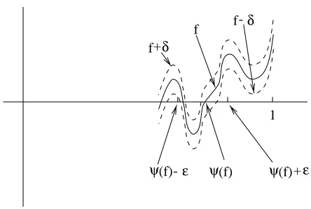
and define a functiong:I →[0,1] by setting
g(x) = sup{s∈[0,1] :B(s) =x}.
It is easy to check that a.s. the interval I is non-degenerate, g is strictly decreasing, left continuous and satisfies B(g(x)) = x. Furthermore, a.s. the set of discontinuities of g is dense in I since a.s. B has no interval of monotonicity. We restrict our attention to the event of probability 1 on which these assertions hold. Let
Vn={x∈I:g(x−h)−g(x)> nhfor some h∈(0, n−1)}.
Sincegis left continuous and strictly deceasing, one readily verifies thatVnis open; it is also dense inI as every point of discontinuity ofg is a limit from the left of points ofVn.By the Baire category theorem,V :=TnVnis uncountable and dense inI.Now ifx∈V then there is a sequence xn ↑x such that g(xn)−g(x)> n(x−xn).Setting t=g(x) and tn =g(xn) we havetn↓tand tn−t > n(B(t)−B(tn)),from which it follows thatD∗B(t)≥0.On the other hand D∗B(t)≤0 since B(s)≤B(t) for alls∈(t,1),by definition of t=g(x).
Exercise7.2. Letf ∈C([0,1]).Prove thatB(t) +f(t) is nowhere differentiable almost surely.
Is the “typical” function inC([0,1]) nowhere differentiable? It is an easy application of the Baire category theorem to show that nowhere differentiability is a generic property for
Lebesgue measure 1. We consider a related idea proposed by Christensen (1972) and by Hunt, Sauer and Yorke (1992). Let X be a separable Banach space. Say that A ⊂ X is
prevalent if there exists a Borel probability measure µ on X such that µ(x+A) = 1 for everyx∈X. A set is callednegligible if its complement is prevalent.
Proposition 7.3. If A1, A2, . . . are negligible subsets of X then Si≥1Ai is also
negli-gible.
Proof. For eachi≥1 letµAi be a Borel probability measure satisfyingµAi(x+Ai) = 0
for all x ∈ X. Using separability we can find for each i a ball Di of radius 2−i centered at xi ∈ X with µAi(Di) > 0. Define probability measures µi, i ≥ 1, by setting µi(E) =
µAi(E +xi|Di) for each Borel set E, so that µi(x+Ai) = 0 for all x and for all i. Let
(Yi;i ≥ 0) be a sequence of independent random variables with dist(Yi) = µi. For all i we have µi[|Yi| ≤ 2−i] = 1. Therefore, S = PiYi converges almost surely. Writing µ for the distribution of S and putting νj = dist(S−Yj),we have µ = µj ∗νj, and hence
µ(x+Aj) =µj∗νj(x+Aj) = 0 for allx and for allj.Thusµ(x+∪i≥1Ai) = 0 for allx. Proposition 7.4. A subsetA of Rdis negligible iff Ld(A) = 0.
Proof. (⇒) Assume A is negligible. Let µA be a (Borel) probability measure such that µA(x+A) = 0 for all x∈ Rd.Since Ld∗µA=Ld (indeed Ld∗µ=Ld for any Borel probability measure µonRd) we have 0 =Ld∗µA(x+A) =Ld(x+A) for all x∈Rd.
(⇐) If Ld(A) = 0 then the restriction of Ld to the unit cube is a probability measure which vanishes on every translate ofA.
Remark. It follows from Exercise 7.2 that the set of nowhere differentiable functions is prevalent in C([0,1]).
8. Strong Markov property and the reflection principle
For each t≥0 let F0(t) =σ{B(s) :s≤t} be the smallestσ-field making every B(s), s≤t,measurable, and setF+(t) =∩u>tF0(u) (the right-continuous filtration). It is known (see, for example, Durrett (1996), Theorem 7.2.4) that F0(t) and F+(t) have the same completion. A filtration {F(t)}t≥0 is a Brownian filtration if for all t ≥ 0 the process {B(t+s)−B(t)}s≥0 is independent of F(t) and F(t) ⊃ F0(t).A random variable τ is a
stopping time for a Brownian filtration {F(t)}t≥0 if {τ ≤ t} ∈ F(t) for all t. For any random timeτ we define the pre-τ σ-field
F(τ) :={A:∀t, A∩ {τ ≤t} ∈ F(t)}.
Proposition 8.1. (Markov property) For everyt≥0 the process {B(t+s)−B(t)}s≥0
is standard Brownian motion independent of F0(t) and F+(t).
It is evident from independence of increments that {B(t+s)−B(t)}s≥0 is standard Brownian motion independent of F0(t).That this process is independent of F+(t) follows from continuity; see, e.g., Durrett (1996, 7.2.1) for details.
8. STRONG MARKOV PROPERTY AND THE REFLECTION PRINCIPLE 19
Theorem 8.2. Suppose that τ is a stopping time for the Brownian filtration{F(t)}t≥0. Then{B(τ +s)−B(τ)}s≥0 is Brownian motion independent of F(τ).
Sketch of Proof. Suppose first thatτ is an integer valued stopping time with respect to a Brownian filtration{F(t)}t≥0.For each integerj the event{τ =j}is inF(j) and the process {B(t+j)−B(j)}t≥0 is independent ofF(j),so the result follows from the Markov property in this special case. It also holds if the values of τ are integer multiples of some
ε > 0, and approximating τ by such discrete stopping times gives the conclusion in the general case. See, e.g., Durrett (1996, 7.3.7) for more details.
One important consequence of the strong Markov property is the following:
Theorem 8.3 (Reflection Principle). Ifτ is a stopping time then B∗(t) :=B(t)1(t≤τ)+ (2B(τ)−B(t))1(t>τ) (Brownian motion reflected at timeτ) is also standard Brownian motion.
Proof. We shall use an elementary fact:
Lemma8.4. LetX, Y, Zbe random variables withX, Y independent and X, Z indepen-dent. IfY ≡d Z then (X, Y)≡d (X, Z).
The strong Markov property states that {B(τ +t) −B(τ)}t≥0 is Brownian motion independent ofF(τ),and by symmetry this is also true of{−(B(τ+t)−B(τ))}t≥0.We see from the lemma that
({B(t)}0≤t≤τ,{B(t+τ)−B(τ)}t≥0) d
≡({B(t)}0≤t≤τ,{(B(τ)−B(t+τ))}t≥0), and the reflection principle follows immediately.
Remark. Consider τ = inf{t : B(t) = max0≤s≤1B(s)}. Almost surely {B(τ +t)− B(τ)}t≥0 is non-positive on some right neighborhood of t= 0, and hence is not Brownian motion. The strong Markov property does not apply here becauseτ is not a stopping time for any Brownian filtration. We will later see that Brownian motion almost surely has no point of increase. Since τ is a point of increase of the reflected process {B∗(t)},it follows that the distributions of Brownian motion and of{B∗(t)} are singular.
Exercise 8.5. Prove that ifA is a closed set thenτA is a stopping time. Solution. {τA≤t}= T
n≥1
S
s∈[0,t]∩Q
{dist(B(s), A)≤ 1
n} ∈ F0(t).
More generally, if A is a Borel set then the hitting time τA is a stopping time (see Bass (1995)).
SetM(t) = max
0≤s≤tB(s).Our next result says M(t) d
≡ |B(t)|.
Theorem 8.6. Ifa >0, then P[M(t)> a] = 2P[B(t) > a].
Proof. Setτa = min{t≥0 :B(t) = a} and let {B∗(t)} be Brownian motion reflected at τa. Then {M(t) > a} is the disjoint union of the events {B(t) > a} and {M(t) >
9. Local extrema of Brownian motion
Proposition 9.1. Almost surely, every local maximum of Brownian motion is a strict local maximum.
For the proof we shall need
Lemma 9.2. Given two disjoint closed time intervals, the maxima of Brownian motion on them are different almost surely.
Proof. For i = 1,2, let [ai, bi], mi, denote the lower, the higher interval, and the corresponding maximum of Brownian motion, respectively. Note that B(a2) −B(b1) is independent of the pair m1−B(b1) and m2 −B(a2). Conditioning on the values of the random variablesm1−B(b1) and m2−B(a2), the eventm1=m2 can be written as
B(a2)−B(b1) =m1−B(b1)−(m2−B(a2)).
The left hand side being a continuous random variable, and the right hand side a constant, we see that this event has probability 0.
We now prove Proposition 9.1.
Proof. The statement of the lemma holds jointly for all disjoint pairs of intervals with rational endpoints. The proposition follows, since if Brownian motion had a non-strict local maximum, then there were two disjoint rational intervals where Brownian motion has the same maximum.
Corollary 9.3. The set M of times where Brownian motion assumes its local maxi-mum is countable and dense almost surely.
Proof. Consider the function from the set of non-degenerate closed intervals with rational endpoints to Rgiven by
[a, b]7→inf
t≥a:B(t) = max a≤s≤bB(s)
.
The image of this map contains the setM almost surely by the lemma. This shows thatM
is countable almost surely. We already know thatB has no interval of increase or decrease almost surely. It follows that B almost surely has a local maximum in every interval with rational endpoints, implying the corollary.
10. Area of planar Brownian motion paths
We have seen that the image of Brownian motion is always 2 dimensional, so one might ask what its 2 dimensional Hausdorff measure is. It turns out to be 0 in all dimensions; we will prove it for the planar case. We will need the following lemma.
10. AREA OF PLANAR BROWNIAN MOTION PATHS 21
Proof. One proof of this fact relies on (outer) regularity of Lebesgue measure. The proof below is more streamlined.
We may assumeA1 and A2 are bounded. By Fubini’s theorem,
Z
R2
1A1 ∗1−A2(x)dx=
Z
R2
Z
R2
1A1(w)1A2(w−x)dwdx
=
Z
R2
1A1(w)
Z
R2
1A2(w−x)dx
dw
=L2(A1)L2(A2)>0.
Thus1A1∗1−A2(x)>0 on a set of positive area. But1A1∗1−A2(x) = 0 unlessA1∩(A2+x) has positive area, so this proves the lemma.
Throughout this sectionB denote planar Brownian motion. We are now ready to prove L´evy’s theorem on the area of its image.
Theorem 10.2 (L´evy). Almost surely L2(B[0,1]) = 0.
Proof. LetX denote the area ofB[0,1], andM be its expected value. First we check thatM <∞. If a≥1 then
P[X > a]≤2P[|W(t)|>√a/2 for somet∈[0,1] ]≤8e−a/8
whereW is standard one-dimensional Brownian motion. Thus
M =
Z ∞
0 P
[X > a]da≤8
Z ∞
0
e−a/8da+ 1<∞.
Note thatB(3t) and√3B(t) have the same distribution, and hence EL2(B[0,3]) = 3EL2(B[0,1]) = 3M.
Note that we have L2(B[0,3])≤ P2j=0L2(B[j, j+ 1]) with equality if and only if for 0≤ i < j ≤ 2 we have L2(B[i, i+ 1]∩B[j, j+ 1]) = 0. On the other hand, for j = 0,1,2,we have EL2(B[j, j+ 1]) =M and
3M =EL2(B[0,3])≤ 2
X
j=0
EL2(B[j, j+ 1]) = 3M,
whence the intersection of any two of the B[j, j + 1] has measure zero almost surely. In particular,L2(B[0,1]∩B[2,3]) = 0 almost surely.
LetR(x) denote the area ofB[0,1]∩(x+B[2,3]−B(2) +B(1)). If we condition on the values ofB[0,1], B[2,3]−B(2), then in order to evaluate the expected value ofB[0,1]∩B[2,3] we should integrateR(x) where x has the distribution ofB(2)−B(1). Thus
0 =E[L2(B[0,1]∩B[2,3])] = (2π)−1
Z
R2
e−|x|2/2E[R(x)]dx
where we are averaging with respect to the Gaussian distribution of B(2)−B(1). Thus
R(x) = 0 a.s. for L2-almost allx, or, by Fubini, the area of the set where R(x) is positive is a.s. zero. ¿From the lemma we get that a.s.
The observation thatL2(B[0,1]) andL2(B[2,3]) are identically distributed and independent completes the proof thatL2(B[0,1]) = 0 almost surely.
11. Zeros of the Brownian motion
In this section, we start the study of the properties of the zero setZBof one dimensional Brownian motion. We will prove that this set is an uncountable closed set with no isolated points. This is, perhaps, surprising since, almost surely, a Brownian motion has isolated zeros from the left (for instance, the first zero after 1/2) or from the right (the last zero before 1/2). However, according to the next theorem, with probability one, it does not have any isolated zero.
Theorem 11.1. LetB be a one dimensional Brownian motion and ZB be its zero set,
i.e.,
ZB ={t∈[0,+∞) :B(t) = 0}.
Then, a.s., ZB is an uncountable closed set with no isolated points.
Proof. Clearly, with probability one, ZB is closed because B is continuous a.s.. To prove that no point ofZBis isolated we consider the following construction: for each rational
q ∈[0,∞) consider the first zero afterq, i.e.,τq= inf{t > q:B(t) = 0}. Note thatτq<∞ a.s. and, since ZB is closed, the inf is a.s. a minimum. By the strong Markov property we have that for eachq, a.s. τq is not an isolated zero from the right. But, since there are only countably many rationals, we conclude that a.s., for allq rational,τqis not an isolated zero from the right. Our next task is to prove that the remaining points ofZB are not isolated from the left. So we claim that any 0< t ∈ ZB which is different from τq for all rational
q is not an isolated point from the left. To see this take a sequence qn↑t, qn∈Q. Define
tn=τqn. Clearlyqn≤tn< t(as tn is not isolated from the right) and so tn↑ t. Thust is
not isolated from the left.
Finally, recall (see, for instance, Hewitt-Stromberg, 1965) that a closed set with no isolated points is uncountable and this finishes the proof.
11.1. General Markov Processes. In this section, we define general Markov pro-cesses. Then we prove that Brownian motion, reflected Brownian motion and a process that involves the maximum of Brownian motion are Markov processes.
Definition 11.2. A function p(t, x, A), p : R×Rd× B → R, where B is the Borel
σ-algebra in Rd, is a Markov transition kernel provided
(1) p(·,·, A) is measurable as a function of (t, x), for eachA∈ B, (2) p(t, x,·) is a Borel probability measure for allt∈Rand x∈Rd, (3) ∀A∈ B, x∈Rd and t, s >0,
p(t+s, x, A) =
Z
Rd
p(t, y, A)p(s, x, dy).
Definition11.3. A process{X(t)}is a Markov process withtransition kernelp(t, x, A) if for allt > s and Borel setA∈ B we have
11. ZEROS OF THE BROWNIAN MOTION 23
The next two examples are trivial consequences of the Markov Property for Brownian motion.
Example11.4. Ad-dimensional Brownian motion is a Markov process and its transition kernelp(t, x,·) hasN(x, t) distribution in each component.
Suppose Z hasN(x, t) distribution. Define |N(x, t)|to be the distribution of|Z|. Example 11.5. The reflected one-dimensional Brownian motion |B(t)| is a Markov process. Moreover, its kernel p(t, x,·) has|N(x, t)|distribution.
Theorem 11.6 (L´evy, 1948). LetM(t) be the maximum process of a one dimensional Brownian motion B(t), i.e. M(t) = max0≤s≤tB(s). Then, the processY(t) =M(t)−B(t)
is Markov and its transition kernel p(t, x,·)has |N(x, t)|distribution.
Proof. For t > 0, consider the two processes ˆB(t) = B(s+t)−B(s) and ˆM(t) = max0≤u≤tBˆ(u). Define FB(s) = σ(B(t),0≤t≤s). To prove the theorem it suffices to check that conditional onFB(s) andY(s) =y, we haveY(s+t)=d |y+ ˆB(t)|.
To prove the claim note thatM(s+t) =M(s)∨(B(s) + ˆM(t)), and so we have
Y(s+t) =M(s)∨(B(s) + ˆM(t))−(B(s) + ˆB(t)).
Using the fact thata∨b−c= (a−c)∨(b−c), we have
Y(s+t) =Y(s)∨Mˆ(t)−Bˆ(t).
To finish, it suffices to check, for everyy ≥0, that y∨Mˆ(t)−Bˆ(t) =d |y+ ˆB(t)|. For any
a≥0 write
P(y∨Mˆ(t)−Bˆ(t)> a) =I+II,
whereI =P(y−Bˆ(t)> a) and
II =P(y−Bˆ(t)≤aand ˆM(t)−Bˆ(t)> a).
Since ˆB=d −Bˆ we have
I =P(y+ ˆB(t)> a).
To study the second term is useful to define the ”time reversed” Brownian motion
W(u) = ˆB(t−u)−Bˆ(t),
for 0 ≤u≤t. Note thatW is also a Brownian motion for 0≤u ≤t since it is continuous and its finite dimensional distributions are Gaussian with the right covariances.
Let MW(t) = max0≤u≤tW(u). Then MW(t) = ˆM(t)−Bˆ(t). SinceW(t) =−Bˆ(t), we have:
II=P(y+W(t) ≤aand MW(t)> a).
If we use the reflection principle by reflectingW(u) at the first time it hitsawe get another Brownian motionW∗(u). In terms of this Brownian motion we haveII=P(W∗(t)≥a+y). Since W∗ =d −Bˆ, it follows II = P(y+ ˆB(t) ≤ −a). The Brownian motion ˆB(t) has continuous distribution, and so, by adding I andII, we get
P(y∨Mˆ(t)−Bˆ(t)> a) =P(|y+ ˆB(t)|> a).
Proposition 11.7. Two Markov processes inRd with continuous paths, with the same initial distribution and transition kernel are identical in law.
Outline of Proof. The finite dimensional distributions are the same. From this we deduce that the restriction of both processes to rational times agree in distribution. Finally we can use continuity of paths to prove that they agree, as processes, in distribution (see Freedman 1971 for more details).
Since the processY(t) is continuous and has the same distribution as |B(t)|(they have the same Markov transition kernel and same initial distribution) this proposition implies {Y(t)}=d {|B(t)|}.
11.2. Hausdorff dimension of ZB. We already know that ZB is an uncountable set with no isolated points. In this section, we will prove that, with probability one, the Hausdorff dimension of ZB is 1/2. It turns out that it is relatively easy to bound from below the dimension of the zero set ofY(t) (also known as set of record values ofB). Then, by the results in the last section, this dimension must be the same of ZB since these two (random) sets have the same distribution.
Definition11.8. A timetis a record time forB ifY(t) =M(t)−B(t) = 0, i.e., iftis a global maximum from the left.
The next lemma gives a lower bound on the Hausdorff dimension of the set of record times.
Lemma 11.9. With probability 1, dim{t∈[0,1] :Y(t) = 0} ≥1/2.
Proof. SinceM(t) is an increasing function, we can regard it as a distribution function of a measureµ, withµ(a, b] =M(b)−M(a). This measure is supported on the set of record times. We know that, with probability one, the Brownian motion is H¨older continuous with any exponent α <1/2. Thus
M(b)−M(a)≤ max
0≤h≤b−aB(a+h)−B(a)≤Cα(b−a) α,
where α < 1/2 and Cα is some random constant that doesn’t depend on a or b. By the Mass Distribution Principle, we get that, a.s., dim{t∈[0,1] : Y(t) = 0} ≥α. By choosing a sequenceαn↑1/2 we finish the proof.
Recall that the upper Minkowski dimension of a set is an upper bound for the Hausdorff dimension. To estimate the Minkowski dimension ofZB we will need to know
P(∃t∈(a, a+ǫ) :B(t) = 0). (11.1) This probability can be computed explicitly and we will leave this as an exercise.
Exercise 11.10. Compute (11.1).
Solution. Conditional onB(a) =x >0 we have
P(∃t∈(a, a+ǫ) :B(t) = 0|B(a) =x) =P( min
a≤t≤a+ǫB(t)<0|B(a) =x).
But the right hand side is equal to
P( max
11. ZEROS OF THE BROWNIAN MOTION 25
using the reflection principle.
By considering also the case wherexis negative we get
P(∃t∈(a, a+ǫ) :B(t) = 0) = 4
Computing this last integral explicitly, we get
P(∃t∈(a, a+ǫ) :B(t) = 0) = 2
πarctan
r
ǫ a.
However, for our purposes, the following estimate will suffice.
Lemma 11.11. For any a, ǫ >0 we have
P(∃t∈(a, a+ǫ) :B(t) = 0)≤C r
ǫ a+ǫ, for some appropriate positive constantC.
Proof. Consider the eventA given by|B(a+ǫ)| ≤√ǫ. By the scaling property of the Brownian motion, we can give the upper bound
P(A) =P
However, knowing that Brownian motion has a zero in (a, a+ǫ) makes the event A very likely. Indeed, we certainly have
P(A)≥P(Aand 0∈B[a, a+ǫ]),
and the strong Markov property implies that
P(A)≥c˜P(0∈B[a, a+ǫ]), (11.3) where
˜
c= min
a≤t≤a+ǫP(A|B(t) = 0). Because the minimum is achieved when t=a, we have
˜
c=P(|B(1)| ≤1)>0,
by using the scaling property of the Brownian motion. From inequalities (11.2) and (11.3), we conclude
P(0∈B[a, a+ǫ])≤ 2
For any, possibly random, closed set A⊂[0,1], define a function
Nm(A) =
special case whereA=ZB we have
The next lemma shows that estimates on the expected value of Nm(A) will give us bounds on the Minkowski dimension (and hence on the Hausdorff dimension).
Lemma 11.12. Suppose A is a closed random subset of [0,1]such that
ENm(A)≤c2mα, forǫ >0. Then, by the monotone convergence theorem,
E Letǫ→0 through some countable sequence to get
dimM(A)≤α, a.s.. And this completes the proof of the lemma.
To get an upper bound on the Hausdorff dimension ofZB note that
ENm(ZB)≤C This implies immediately dimH(ZB)≤1/2 a.s. Combining this estimate with Lemma 11.9 we have
Theorem 11.13. With probability one we have
12. HARRIS’ INEQUALITY AND ITS CONSEQUENCES 27
From this proof we can also infer thatH1/2(Z
B) <∞ a.s. Later in the course we will prove thatH1/2(Z
B) = 0. However, it is possible to define a more sophisticatedϕ-Hausdorff measure for which, with probability one, 0<Hϕ(Z
B)<∞. Such a function ϕis called an exact Hausdorff measure function forZB.
12. Harris’ Inequality and its consequences
We begin this section by proving Harris’ inequality.
Lemma12.1 (Harris’ inequality). Suppose thatµ1, . . . , µdare Borel probability measures
on R and µ = µ1×µ2 ×. . .×µd. Let f, g : Rd → R be measurable functions that are
provided the above integrals are well-defined.
Proof. One can argue, using the Monotone Convergence Theorem, that it suffices to prove the result when f andg are bounded. We assumef andg are bounded and proceed by induction. Suppose d= 1. Note that
(f(x)−f(y))(g(x)−g(y))≥0
and (12.1) follows easily. Now, suppose (12.1) holds ford−1. Define
f1(x1) =
Z
Rd−1
f(x1, . . . , xd)dµ(x2). . . dµd(xd),
and define g1 similarly. Note that f1(x1) and g1(x1) are non-decreasing functions of x1. Since f and g are bounded, we may apply Fubini’s Theorem to write the left hand side of (12.1) as by using the result for the d= 1 case we can bound (12.2) below by
Z
which equals the right hand side of (12.1), completing the proof.
Example 12.3. Let X1, . . ., Xn be an i.i.d. sample, where each Xi has distribution
µ. Given any (x1, . . . , xn) ∈ Rn, define the relabeling x(1) ≥ x(2) ≥ . . . ≥ x(n). Fix i and j, and define f(x1, . . . , xn) = x(i) and g(x1, . . . , xn) = x(j). Then f and g are measurable and nondecreasing in each component. Therefore, if X(i) and X(j) denote the ith and jth order statistics of X1, . . . , Xn, then it follows from Harris’ Inequality that E[X(i)X(j)] ≥ E[X(i)]E[X(j)], provided these expectations are well-defined. See Lehmann (1966) and Bickel (1967) for further discussion.
For the rest of this section, let X1, X2, . . . be i.i.d. random variables, and let Sk =
Pk
i=1Xi be their partial sums. Denote
pn=P(Si≥0 for all 1≤i≤n). (12.3) Observe that the event that {Sn is the largest amongS0, S1, . . . Sn} is precisely the event that the reversed random walkXn+. . .+Xn−k+1 is nonnegative for allk= 1, . . ., n; thus this event also has probability pn. The following theorem gives the order of magnitude of
pn.
Theorem12.4. If the incrementsXi have a symmetric distribution (that is,Xi =d −Xi)
or have mean zero and finite variance, then there are positive constants C1 and C2 such that C1n−1/2 ≤pn≤C2n−1/2 for all n≥1.
Proof. For the general argument, see Feller (1966), Section XII.8. We prove the result here for the simple random walk, that is when each Xi takes values ±1 with probability half each.
Define the stopping time τ−1 = min{k:Sk=−1}. Then
pn=P(Sn≥0)−P(Sn≥0, τ−1< n). Let{Sj∗} denote the random walk reflected at timeτ−1, that is
Sj∗=Sj forj≤τ−1, Sj∗= (−1)−(Sj+ 1) forj > τ−1. Note that ifτ−1 < nthen Sn≥0 if and only ifSn∗ ≤ −2, so
pn=P(Sn≥0)−P(Sn∗ ≤ −2). Using symmetry and the reflection principle, we have
pn=P(Sn≥0)−P(Sn≥2) =P(Sn∈ {0,1}), which means that
pn = P(Sn= 0) = n/n2
2−n forneven, pn = P(Sn= 1) = (n−n1)/22−n fornodd.
Recall that Stirling’s Formula givesm!∼√2πmm+1/2e−m, where the symbol∼means that the ratio of the two sides approaches 1 asm→ ∞. One can deduce from Stirling’s Formula that
pn∼
r
2
πn,
13. POINTS OF INCREASE FOR RANDOM WALKS AND BROWNIAN MOTION 29
The following theorem expresses, in terms of thepi, the probability thatSjstays between 0 andSn forj between 0 andn. It will be used in the next section.
Theorem 12.5. We have p2n≤P(0≤Sj ≤Sn for all 1≤j ≤n)≤p2⌊n/2⌋. Proof. The two events
A = {0≤Sj for all j ≤n/2} and
B = {Sj ≤Sn for j≥n/2}
are independent, since A depends only on X1, . . ., X⌊n/2⌋ and B depends only on the re-mainingX⌊n/2⌋+1, . . . , Xn. Therefore,
P(0≤Sj ≤Sn)≤P(A∩B) =P(A)P(B)≤p2⌊n/2⌋, which proves the upper bound.
For the lower bound, we follow Peres (1996) and letf(x1, . . . , xn) = 1 if all the partial sumsx1+. . .+xk fork= 1, . . ., nare nonnegative, and f(x1, . . . , xn) = 0 otherwise. Also, define g(x1, . . . , xn) = f(xn, . . ., x1). Then f and g are nondecreasing in each component. Letµj be the distribution of Xj, and letµ=µ1×. . .×µn. By Harris’ Inequality,
Z
Rn
f g dµ≥ Z
Rn
f dµ Z
Rn
g dµ
=p2n.
Also,
Z
Rn
f g dµ =
Z
Rn
1{for allj, x1+. . .+xj ≥0 and xj+1+. . .+xn≥0}dµ = P(0≤Sj ≤Sn for all 1≤j≤n),
which proves the lower bound.
13. Points of increase for random walks and Brownian motion
The material in this section has been taken, with minor modifications, from Peres (1996). A real-valued function f has a global point of increase in the interval (a,b) if there is a point t0 ∈(a, b) such that f(t)≤f(t0) for all t∈(a, t0) and f(t0)≤f(t) for all t∈(t0, b). We sayt0 is alocal point of increaseif it is a global point of increase in some interval. Dvoretzky, Erd˝os and Kakutani (1961) proved that Brownian motion almost surely has no global points of increase in any time interval, or, equivalently, that Brownian motion has no local points of increase. Knight (1981) and Berman (1983) noted that this follows from properties of the local time of Brownian motion; direct proofs were given by Adelman (1985) and Burdzy (1990). Here we show that the nonincrease phenomenon holds for arbitrary symmetric random walks, and can thus be viewed as a combinatorial consequence of fluctuations in random sums.
Definition. Say that a sequence of real numberss0, s1, . . . , sn has a (global)point of
Theorem 13.1. LetS0, S1, . . ., Sn be a random walk where the i.i.d. increments Xi =
Si−Si−1 have a symmetric distribution, or have mean 0 and finite variance. Then
P(S0, . . ., Sn has a point of increase)≤
C
logn , for n >1, where C does not depend onn.
We will now see how this result implies the following
Corollary 13.2. Brownian motion almost surely has no points of increase.
Proof. To deduce this, it suffices to apply Theorem 13.1 to a simple random walk on the integers. Indeed it clearly suffices to show that the Brownian motion{B(t)}t≥0 almost surely has no global points of increase in a fixed rational time interval (a, b). Sampling the Brownian motion when it visits a lattice yields a simple random walk; by refining the lattice, we may make this walk as long as we wish, which will complete the proof. More precisely, for any vertical spacing h >0 define τ0 to be the firstt ≥a such that B(t) is an integral multiple of h, and for i ≥0 let τi+1 be the minimal t ≥ τi such that |B(t)−B(τi)|= h. Define Nb = max{k∈Z:τk≤b}. For integers isatisfying 0≤i≤Nb, define
Si =
B(τi)−B(τ0)
h .
Then, {Si}Ni=1b is a finite portion of a simple random walk. If the Brownian motion has a (global) point of increase in (a, b) att0, and ifkis an integer such thatτk−1 ≤t0 ≤τk, then this random walk has points of increase at k−1 and k. Such a k is guaranteed to exist if |B(t0)−B(a)|> hand |B(t0)−B(b)|> h. Therefore, for all n,
P( Brownian motion has a global point of increase in (a, b)) (13.1) ≤ P(Nb≤n) +P(|B(t0)−B(a)| ≤h) +P(|B(t0)−B(b)| ≤h)
+ ∞
X
m=n+1
P(S0, . . . , Smhas a point of increase, and Nb =m).
Note thatNb ≤nimplies |B(b)−B(a)| ≤(n+ 1)h, so
P(Nb≤n)≤P(|B(b)−B(a)| ≤(n+ 1)h) =P
|Z| ≤ (√n+ 1)h b−a
,
whereZ has a standard normal distribution. Since S0, . . ., Sm, conditioned onNb =m is a finite portion of a simple random walk, it follows from Theorem 13.1 that for some constant
C, we have
∞
X
m=n+1
P(S0, . . . , Smhas a point of increase, and Nb =m)
≤ ∞
X
m=n+1
P(Nb =m)
C
logm ≤ C
log(n+ 1).
13. POINTS OF INCREASE FOR RANDOM WALKS AND BROWNIAN MOTION 31
To prove Theorem 13.1, we prove first
Theorem 13.3. For any random walk {Sj} on the line,
P(S0, . . . , Sn has a point of increase)≤2
Pn
k=0pkpn−k
P⌊n/2⌋ k=0 p2k
. (13.2)
Proof. The idea is simple. The expected number of points of increase is the numerator in (13.3), and given that there is at least one such point, the expected number is bounded below by the denominator; the ratio of these expectations bounds the required probability. To carry this out, denote byIn(k) the event thatkis a point of increase forS0, S1, . . ., Sn and by Fn(k) =In(k)\ ∪ik=0−1In(i) the event that kis the first such point. The events that {Sk is largest among S0, S1, . . . Sk} and that {Sk is smallest among Sk, Sk+1, . . .Sn} are independent, and thereforeP(In(k)) =pkpn−k.
Observe that ifSjis minimal amongSj, . . ., Sn, then any point of increase forS0, . . . , Sj is automatically a point of increase for S0, . . . , Sn. Therefore forj≤k we can write
Fn(j)∩In(k) =
Fj(j) ∩ {Sj ≤Si≤Skfor alli∈[j, k]} ∩ {Sk is minimal amongSk, . . . , Sn}.
The three events on the right-hand side are independent, as they involve disjoint sets of summands; the second of these events is of the type considered in Theorem 12.5. Thus,
P(Fn(j)∩In(k)) ≥ P(Fj(j))p2k−jpn−k
≥ p2k−jP(Fj(j))P(Sj is minimal amongSj, . . . , Sn) ,
sincepn−k≥pn−j. Here the two events on the right are independent, and their intersection is precisely Fn(j). Consequently P(Fn(j)∩In(k)) ≥ p2k−jP(Fn(j)).
Decomposing the event In(k) according to the first point of increase gives
n
X
k=0
pkpn−k = n
X
k=0
P(In(k)) = n
X
k=0 k
X
j=0
P(Fn(j)∩In(k))
≥ ⌊n/X2⌋
j=0
j+X⌊n/2⌋
k=j
p2k−jP(Fn(j)) ≥ ⌊n/X2⌋
j=0
P(Fn(j)) ⌊n/X2⌋
i=0
p2i . (13.3)
Proof of Theorem 13.1. To bound the numerator in (13.3), we can use symmetry to deduce from Theorem 12.4 that
n
which is bounded above because the last sum isO(n1/2). Since Theorem 12.4 implies that the denominator in (13.2) is at leastC12log⌊n/2⌋, this completes the proof.
The following theorem shows that we can obtain a lower bound on the probability that a random walk has a point of increase that differs from the upper bound only by a constant factor.
Theorem 13.4. For any random walk on the line,
P(S0, . . . , Sn has a point of increase)≥
In particular if the increments have a symmetric distribution, or have mean 0 and finite variance, then P(S0, . . . , Sn has a point of increase)≍1/lognforn >1, where the symbol ≍ means that the ratio of the two sides is bounded above and below by positive constants that do not depend on n.
Proof. Using (13.3), we get
This implies (13.4). The assertion concerning symmetric or mean 0, finite variance walks follows from Theorem 12.4 and the proof of Theorem 13.1.