David Clingingsmith is Assistant Professor of Economics in the Weatherhead School of Management at Case Western Reserve University. He is grateful for discussions with Leah Platt Boustan, Carola Frydman, Silke Forbes, Claudia Goldin, Susan Helper, Eric Hilt, Lakshmi Iyer, Asim Khwaja, Michael Kremer, Bob Margo, Rohini Pande, Jim Rebitzer, Heather Royer, Scott Shane, Justin Sydnor, Mark Votruba, and Jeffrey Williamson. This paper has benefi ted from comments by participants at the Harvard Economic History Workshop, the Harvard- Hitotsubashi- Warwick conference on Economic Change around the Indian Ocean, the 2008 Canadian Network for Economic History conference, the 36th Annual Conference on South Asia, the 45th Cliometrics Conference, and seminar audiences at University of California Davis, University of Toronto, Vanderbilt, Reed College, Case Western Reserve University, and the University of British Colum-bia. He also thanks three anonymous JHR referees for valuable suggestions. The data used in this article can be obtained beginning August 2014 through July 2017 from David Clingingsmith, 11119 Bellfl ower Road, Cleveland, Ohio. Email: david.clingingsmith@case .edu.
[Submitted November 2011; accepted December 2012]
ISSN 0022- 166X E- ISSN 1548- 8004 © 2014 by the Board of Regents of the University of Wisconsin System
T H E J O U R N A L O F H U M A N R E S O U R C E S • 49 • 1
in India
David Clingingsmith
A B S T R A C T
Bilingualism is a distinct and important form of human capital in linguistically diverse countries. When communication among workers increases productivity, there can be economic incentives to learn a second language. I study how the growth of industrial employment increased bilingualism in India between 1931 and 1961. During that period, Indian factories were linguistically mixed. I exploit industrial clustering and sectoral demand growth for identifi cation. The effect on bilingualism was strongest in import- competing districts and among local linguistic minorities. Bilingualism was mainly the result of learning, rather than than migration or assimilation, and was not a byproduct of becoming literate. My results shed new light on human capital investment in developing economies and on the long- run evolution of languages and cultures.
I. Introduction
income countries where most people speak the same mother tongue.1 In linguistically
diverse societies—such as India, Indonesia, Nigeria, and the Philippines—language differences create real barriers to communication and exchange. Each of these coun-tries are home to hundreds of sizeable language communities.2 People who speak
an uncommon language may fi nd their prospects for employment or trade limited relative to speakers of a common language. Investing in a second language may con-fer economic benefi ts by expanding the capacity to communicate. Despite the large populations in linguistically diverse countries, we are only beginning to learn about the investment in and returns to language skills.
This paper studies the relationship between the expansion of the modern sector and bilingualism in India between 1931 and 1961. This period spans the beginning of mod-ern economic growth in India. Industrial jobs more than doubled, spurred in part by strong increases in tariffs. Most of the new jobs were in larger factories that exploited scale economies through task specialization and mechanization. India is linguistically diverse even within local labor markets, and large factories mixed workers of different mother tongues in their shops and departments.
While this period of Indian history provides a good environment to study whether industrial employment can lead to increased investment in bilingualism, its primary advantage is the availability of high- quality data. India is the only linguistically di-verse country to have regularly collected census data on bilingualism. Tabulations of bilingualism were published at the district level in 1931 and 1961. District- level data enables the use of within- state variation, a great advantage because education and industrial policy is set at the state level. I created a new data set that contains information on district- level economic outcomes and languages spoken. The available tabulations cover most of the country.3 Data on multiple languages per district allows
me to study the growth in bilingualism for mother tongue speakers of majority and minority languages separately.
The empirical analysis centers on estimating how changes in the industrial share of employment affects the share of the population that is bilingual. I estimate this effect in fi rst differences and include state fi xed effects.4 There are several reasons why OLS
estimation may not identify the true effect of industrial growth. First, a change in how the census counted workers induces substantial measurement error in the industrial share and creates a downward bias in the OLS. Second, literacy is positively corre-lated with the industrial share and bilingualism, producing a positive bias in the OLS estimate. While I have a measure for literacy, it cannot be a used as control because, as a form of human capital, it is endogenous.
I create an instrumental variable to provide consistent estimates of the industrial share effect. I collect data on employment shares for 14 industrial sectors, such as tex-tiles and chemicals, for each district in 1931. The instrument is computed by making the counterfactual assumption that, for each district, the 14 industrial sectors grow at their national average rate. This assumption holds the 1931 sectoral structure for each dis-trict constant and applies the average rate of employment growth in those sectors to the
1. A person’s mother tongue is the primary language they learned in childhood. 2. I defi ne sizeable as having more than 10,000 speakers.
3. In India the district is the administrative level below the state. The average district in my data is about 70 miles square and had a 1931 population of 1.5 million people.
district. The predicted change in the industrial share under the counterfactual assump-tion is the instrument. This approach was pioneered by Bartik (1991) and Blanchard and Katz (1992) and has had several recent applications (Autor and Duggan 2003; Lutt mer 2005; Card 2009; Lewis 2011). To compute the instrument for a particular dis-trict d, I regress the actual change in the industrial share on the 1931 sectoral shares for the districts other than d. The instrument is an out- of- sample prediction for district d. Instrumental variables estimation fi nds that industrial growth has a strong positive effect on bilingualism. A one- point increase in the industrial share raises the bilingual share by 1.61 points. This effect is much larger than the OLS estimate of 0.55 points. The effect is 2.09 points for speakers of a district’s minority languages, which is con-sistent with the greater potential bilingualism has to increase the set of individuals with whom they can speak.
The large difference between the OLS and IV estimates refl ects 1) measurement error as discussed above and 2) the source of the identifying variation. IV produces an estimate of the local average treatment effect, or LATE, rather than the average effect (Angrist, Imbens, and Rubin 1996; Angrist and Pischke 2009). However, the large difference also raises the concern of a positive correlation between the instrument and time- varying unobservable determinants of bilingualism. I provide a check on the exogeneity of the instrument by showing it is not correlated with 1931 district characteristics. State fi xed effects eliminate concerns about confounding effects of policy changes. Moreover, IV estimation using this instrument is not particularly sensitive to small violations of the exclusion restriction. I show that if the residual correlation between the instrument and unobservables is 0.2, for example, the IV estimate would be too large by 0.27 points.
In my setting, the LATE is the effect of those changes in the industrial share that resulted from national- level sectoral growth channeled through the existing pattern of industrial location. This expansion in demand will tend to matter more for goods that are traded at the national level. As it happens, industrial growth during the panel was strongly infl uenced by increased tariffs, which favored home production of previ-ously imported goods. Agglomeration economies and proximity to raw materials also promote persistence of the 1931 industrial structure.
Is this interpretation of the LATE refl ected in districts more exposed to trade? I investigate the role of foreign trade by creating a measure of each district’s share in the net value of manufacturing imports. I call above- median districts “import competing.” In import- competing districts, a one- point increase in the industrial share produces a 1.89- point increase in bilingualism, compared to a 0.50- point increase in the other districts. Note that Indian imports were intensive in technically sophisticated goods such as steel, machine tools, petroleum products, and vehicles.
Potential bilinguals must choose the language they will learn. India has two lingua francas, English and Hindi, that are widely used for communication by people with different mother tongues. The dominant language in a district has a 75 percent share, which makes it attractive to minorities. I found that the choice of second language dif-fered for dominant and secondary- language speakers. Mother- tongue speakers of the dominant language in their district were pushed strongly toward learning Hindi and English and away from local minority languages. Mother- tongue speakers of minority languages were pushed most strongly toward English and other languages from the district, with a smaller effect on Hindi.
in-crease the bilingual share. First and central to my argument, people may decide to invest in learning a second language. Second, they may wish to become literate and acquire a second language as part of doing so. Third, speakers of the language may decide to migrate from outside the district to where industry is expanding. Fourth and fi nally, some parents who are bilingual may decide to teach their children only their second language, causing them to assimilate to the other language.
Industrial expansion did lead to higher literacy. The effect was 1.14 points for each point change in the industrial share. It was stronger in the import- competing districts, but the difference was small—1.17 versus 0.92 points. This suggests that industries differed in their relative demand for bilingualism and literacy.
If bilingualism is a step taken to become literate, then some of the effect of in-dustrial growth on bilingualism will be merely a refl ection of investment in literacy. Ideally, we would like to know the effect of industrial growth on bilingualism con-ditional on literacy. Because literacy is endogenous, this would require an adcon-ditional instrument and the interpretative diffi culties associated with two sources of identifying variation. Instead, I explore the sensitivity of the IV estimates to assumptions about the conditional coeffi cient on literacy were it to be included in the regression. Even under the assumption that literacy leads to one- for- one changes in bilingualism, the conditional effect of industrial growth on bilingualism is 0.48 and signifi cantly differ-ent from zero. I also show that a one- point increase in the industrial share raises the number of bilinguals per literate person 13 points. The average growth in the industrial share is 2.9 points. Industrial growth thus increased the number of bilinguals per liter-ate person by approximliter-ately 0.38. Overall, literacy rose faster than bilingualism over the panel, leading the number of bilinguals per literate to fall from from 1.47 to 0.55.
I assess migration by considering effects on surrounding districts, which are a likely source of migrants. I take the set of languages spoken in each district and calculate how many speak that language in the geographically adjacent districts. I also calculate how many are bilingual and the bilingual share. I fi nd that industrial growth has a rela-tively small, statistically insignifi cant negative effect on the bilingual share in adjacent districts. Level regressions show no effect of industrial growth on the overall size of languages in adjacent districts.
Finally, I fi nd that industrial growth doesn’t change the share of the population speaking the majority language or linguistic heterogeneity, which suggests little as-similation is going on. I do fi nd that secondary languages that had higher initial bilin-gualism had lower population shares 30 years later. This patterns holds for districts between 1931 and 1961 and in state- level data between 1961 and 1991.
This paper makes a contribution to several active literatures. It is closely related to recent studies of on the returns to English in India (Munshi and Rosenzweig 2006; Kapur and Chakraborty 2009; Oster and Millett 2010; Shastry 2012; Azam, Chin, and Prakash 2013). This literature takes the growth of IT and business process outsourcing as its point of departure. I show that bilingualism, including in English, has long been valuable in the larger, lower- skilled industrial sector. This fi nding is relevant today because the average skill level of Indian workers remains low and the country remains linguistically fragmented.
An older and larger literature has studied the returns to bilingualism in high- income countries. (Examples include Chiswick and Miller 1995; Dustmann and van Soest 2001; Berman, Lang, and Siniver 2003; Fry and Lowell 2003; Bleakley and Chin 2004; and Lang and Siniver 2009.) The gist of this literature is that returns tend to be large for immigrants who become bilingual in the primary language of their adopted country and near zero for natives who learn a second language. My study relates to both of these strands. First, linguistic minorities in India tend to be small shares of the local population, meaning the challenge they face is similar to that of immigrants. Second, in contrast to the fi ndings for high- income countries, there is a return to bi-lingualism for the linguistic majority in India. This difference probably results from greater linguistic diversity in India, which creates a greater need for a lingua franca than in the high- income countries studied.
Linguistic diversity has been associated with a variety of poor economic outcomes, from low economic growth to low levels of public goods. (See Alesina, Baqir, and Easterly 1999; Alesina et al. 2003; Alesina and La Ferrara 2005.) One root cause for this correlation, among several that have been proposed, is communication barri-ers to exchange. Investment in bilingualism induced by industrialization may be an endogenous response to a diverse environment. While I do not fi nd a direct effect on assimilation or linguistic diversity, my results are still consistent with endogenous changes in linguistic diversity over the long run.
The body of this paper contains fi ve sections. Section II provides information on the Indian economy that supports the empirical analysis. Section III describes the construction of the data set and provides summary statistics. Section IV develops a regression model, discusses the challenges of identifying the parameters, and provides an instrumental variables solution. Section V presents the empirical analysis. Sec-tion VI discusses the implicaSec-tions of the results.
II. Economic Institutions and Language in Context
A. The Expansion of Indian Industry
India’s main industrial sectors in 1931 were textiles, wood products, food processing, and ceramics. Industry made up 8.9 percent of India’s total employment and con-tributed 13.2 percent of its GDP (Sivasubramonian 2000). By 1961, industry was 22.1 percent of GDP and employed 11.8 percent of the work force. (See Figure A1 in the online appendix: http: // jhr.uwpress .org.) The overall number of industrial jobs nearly doubled, and about 70 percent of new jobs were in large- scale industrial en-terprises (Sivasubramonian 2000; India 1962).5 Historical studies have suggested that
increased task specialization was a major reason for the increase in industrial scale during this era (Roy 1999, 2000).
India’s trade policy was an important factor driving industrial growth in this era. In 1919, the government of India was given fi scal autonomy from Britain, which meant it could set tariff policy independently. At the same time, rights to land revenue, the main source of income for the central government, were devolved to the provinces. Thereafter, India’s central government relied increasingly on import tariffs to raise revenue (Tomlinson 1979). Average import tariffs were about 5 percent from 1900 to 1920, then rose steeply to more than 30 percent in the early 1930s. (See Figure A2 in the online appendix: http: // jhr.uwpress .org.) Average tariffs were about 25 percent between 1931 and 1961. The ensuing substitution of domestically produced goods for technologically advanced imports is consistent with industrial growth being mostly in the large- scale sector.
B. The Industrial Labor Market
An understanding of impact new industrial jobs had on bilingualism should be rooted in an understanding of labor market institutions and fi rm organization.
Since the establishment of the fi rst large factories in the mid- 19th century, caste networks have played a central role in connecting industrial fi rms and employees. Castes are endogamous and hereditary social groups to which most Indians belong. Surveys conducted in the 1950s and 1960s reported 30 percent to 50 percent of in-dustrial workers made use of personal contacts, including through caste networks, in getting their jobs (Lambert 1963; Sheth 1968; Holmström 1976). Members of a caste speak the same language, so bilingualism does not play a role in making connections to employers through the caste network.
In their classic studies of the industrial sector in Mumbai, Morris (1965) and Chan-dravarkar (1994) discuss how labor shortages helped entrench a recruitment system based on caste. The key fi gure in this system was the jobber. The jobber used his contacts among members of his caste in the hinterland to muster labor to the factory in the city. Once there, he supervised the recruits in their jobs. The jobber and his workers shared the common language of their caste (in Mumbai this was typically Marathi), although the jobber also spoke the language of the factory owners (typically Gujarati). A similar system of labor recruitment was found in Calcutta jute mills and the tea plantations of Assam (Roy 2010).
When labor became abundant in the city in the early 20th century, the recruiting function shifted to personnel departments and the jobber became more like a foreman (Morris 1965; Chandravarkar 1994; Breman 1999). The jobber’s enduring legacy was the establishment of caste connections as a gateway to industrial employment. Mun-shi and Rosenzweig (2006) found that caste networks and the links they provided to particular occupations continued to infl uence the occupation and education choices of Maharashtrian children in Mumbai in 2001.
C. Bilingualism on the Factory Floor
Once the jobber’s role in recruitment had ended, the linguistic composition of work groups became less constrained. Industrial sociologists have discussed the use of lan-guage in Indian factories in a number of studies. Some have collected detailed data on the language, occupation, and work group of factory employees. This work shows that multilingual work groups were the norm rather than the exception, and workers used second- language skills on the job.
The most vivid picture of language use on the factory fl oor comes from a 1953 study by A.K. Rice (1958) of productivity and social organization in an Ahmedabad textile factory. He observed,
Languages are regional and, although Ahmedabad is in the Gujarat, and the com-mon language of all those who work in the industry is Gujarati, it is not uncom-mon to fi nd three or even four different languages being spoken in the same department of one mill. One one occasion, in a discussion with a group of eight workers, which was being interpreted in three languages, Gujarati, Hindi, and English, it was discovered after half an hour that one worker had not up to that time understood a word that had been said—he came from South India and spoke only Tamil.
Bilingualism played a central role in the interaction described. It is easy to see the potential disadvantage that a worker might face by not being able to engage in such discussions. Rice goes on to describe how language and caste differences had compli-cated efforts to improve productivity.
Sheth (1968) studied an electrical factory in a small Gujarati town in 1958. He documented the distribution of mother tongues within its departments and workshops. (See Table A1 in the online appendix: http: // jhr.uwpress .org.) The factory had 810 workers. A categorical ANOVA shows that 91 percent of the variation in language spoken is within the functional units, rather than across them (Light and Margolin 1971). Sheth noted that employees were in “continuous interaction” with each other when on the factory fl oor. In other words, they needed to talk to do their jobs. A related study of fi ve factories in Poona during the late 1950s found that 20 to 30 percent of employees were not native Marathi speakers (Lambert 1963). The percentages were similar across occupational groups and factories. Similar patterns are described by Gokhale (1957) and Vidyarthi (1970).
rather than across, occupations. There is no segregation of occupations by language groups in the industrial sector as a whole. This fi nding is particularly interesting as it is these very occupations that caste networks enable the Marathi- speaking boys in Munshi and Rosenzweig (2006) to access.
D. The Returns to Bilingualism
Did bilingualism earn a return in the Indian labor market of the era? Addressing this question completely would require data on wages, which do not exist in a useful form. A substantial literature, both within India and beyond, points to large returns to bi-lingualism when the second language is a lingua franca, such as English or Hindi in India, or the dominant language of the country.
Recent studies fi nd substantial returns to bilingualism in English in India. Using individual- level data and conditioning on schooling, Azam, Chin, and Prakash (2013) fi nd a 34 percent return to English fl uency and a 13 percent return to knowing a little English. Kapur and Chakraborty (2009) report on a policy intervention in West Bengal in 1983 that removed English instruction from public primary schools. Using variation across cohorts and districts in English exposure, they fi nd a 68 percent wage premium for English. Shastry (2012) shows that export- oriented IT fi rms, which rely on En-glish speakers to serve clients in the United States, chose to locate in areas where the cost of learning English relative to Hindi were small. The relative costs were based on predetermined language structure. These areas then showed a response in school enrollment growth.
Immigrants to industrial countries earn a large return to fl uency in the language of their new home. In a study that included Australia, Canada, the United States, and Israel, Chiswick and Miller (1995) found returns to English fl uency of 10 percent to 17 percent conditional on schooling. A followup study on West Germany found an effect of German fl uency on wages of 7.3 points per standard deviation of fl uency (Dustmann and van Soest 2001). Berman, Lang, and Siniver (2003) estimated that one- half to three- quarters of the wage convergence for skilled immigrants to Israel came from improved Hebrew. The cost of learning a language increases sharply in adolescence due to biological changes. Bleakley and Chin (2004) use this variation to estimate returns to English for child immigrants to the United States. They fi nd 67 percent higher wages for those who speak English well rather than poorly, though the difference largely comes through increased schooling.
In contrast, Fry and Lowell (2003) fi nd that among native speakers of English there is no additional return to knowing a second language conditional on schooling. How-ever, those monolingual in another language earn 11 percent less, in line with the estimates of Chiswick and Miller (1995). Chiswick and Miller (1998) found similar results. The situation faced by the native born in the United States is similar to that of dominant- language speakers in India.
E. National Markets for Goods and Local Markets for Labor
reduced interregional price disparities in major commodities, and created a national market for industrial goods (Donaldson 2010; Burgess and Donaldson 2010).
Interestingly, migration rates remained quite low well into the late 20th century (Cashin and Sahay 1996). At the end of my panel in 1961, only 3.2 percent of the Indian population were interstate migrants. Even the substantial economic growth induced by India’s 1991 trade liberalization failed to induce substantial cross- district migration (To-palova 2010). Endogamous marriage patterns and geographic concentration among In-dia’s castes are important in explaining low migration (Munshi and Rosenzweig 2009). Borjas (2003) and subsequent literature highlighted the problem of identifying the impact of labor supply shocks from immigration in the United States by using geo-graphic variation across local labor markets. Labor markets in the United States are well integrated, and local shocks diffuse quickly. If Indian labor markets were as well integrated, it would be impossible to disentangle the migration and learning chan-nels through which industrial employment growth would increase bilingualism in a particular region.
F. Bilingualism, Literacy, and Education
Bilingualism and literacy are related forms of human capital both in a functional sense and in the way they are acquired. Bilingualism enables face- to- face communication among people with different mother tongues, while literacy enables communication across time and space between people who share a written language. The census con-sidered a person to be literate if they were able to read and respond to a simple letter India (1933a). Bilingualism required regular use of more than one language. In other words, the criteria were for capacity in the case of literacy and use for bilingualism. In 1931, 8 percent of the Indian population was bilingual and 9 percent was literate. Bilingualism had increased 50 percent and literacy 300 percent by 1961.
Functional literacy and bilingualism can be acquired in school or through indepen-dent effort. The population share of primary school completers was only 8.1 percent as late as 1960 (Barro and Lee 2010). While formal schooling in the vernacular languages of India and in English had been promoted since the 1850s, per capita spending on primary education and enrollment rates in British India were consistently among the lowest in the world (Chaudhary 2009). Literacy is much higher than primary comple-tion in 1961 (27 percent versus 8 percent), which is consistent with basic literacy re-quiring only a small amount of classroom time and with learning taking place outside the classroom. It isn’t possible to directly assess how much of the growth of either literacy or bilingualism resulted from formal schooling and how much resulted from other means because the Census of India did not ask about schooling independent of literacy or bilingualism until 1941 (Srivastava 1972).
tradeoff about where to invest their effort. As it turns out, increases in bilingualism and literacy are only weakly correlated with ρ = 0.16. This, along with low rates of primary completion, points to a decoupling of the production of literacy and bilingual-ism in this period and a limited role for formal schooling.
III. Data and Summary Statistics
A. Construction of the Data Set
To conduct the analysis, I constructed a panel data set of Indian districts for the years 1931 and 1961 from published tables of the Census of India (India 1933a, 1962). Each census was a complete enumeration of the population.
The data set contains information at the district level on economic variables. Within each district, I have disaggregated information by language on the number of speakers and bilinguals. I refer to observations at this level as a district- language. This clas-sifi cation precludes double counting.
The Censuses recorded the language names reported by respondents. Languages often have locally specifi c names and must be aggregated to consistent categories. The category scheme used in 1961 was fi ner grained, and the category names were changed in some cases. I matched language categories by hand on a district- by- district basis using Ethnologue, a comprehensive global database of languages that includes alternative names and dialects (Gordon 2005).
There were substantial changes in district boundaries between 1931 and 1961. Fol-lowing India’s independence from Britain in 1947, hundreds of sovereign princely states were integrated into the existing colonial administrative framework inherited by India. A reorganization of state boundaries in the 1950s led to further changes in district boundaries. I used maps and a concordance to generate a mapping of all British districts and the princely states that fall within India’s 1961 boundaries into consistent geographical units (Singh and Banthia 2004). Implications of the boundary changes for the analysis are discussed in Section IV.
I restrict the data set to districts in which adequate data on bilingualism was reported in 1931. While the census form was standard in that year, the published volumes were prepared at the provincial level and do not always contain the same tables. There is no evidence that the complete data was not collected. Each district has an average of fi ve language observations.
The data set contains 137 districts and covers present- day India excluding Uttar Pradesh, Punjab, Himachal Pradesh, Rajasthan, and portions of Bihar, which are the states where the bilingualism data were unavailable. Taken together, these excluded states are substantially less urban, more agricultural, less literate, and less bilingual than the others. They are also less linguistically diverse. We therefore need to take care in extrapolating the results to the rest of India.
B. Characteristics of Districts and Their Languages
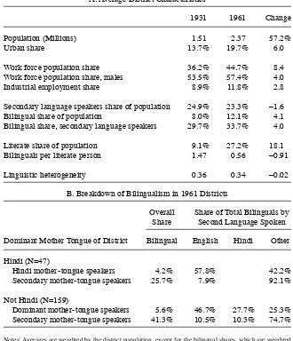
Table 1
Summary Statistics
A. Average District Characteristics
1931 1961 Change
Population (Millions) 1.51 2.37 57.2%
Urban share 13.7% 19.7% 6.0
Work force population share 36.2% 44.7% 8.4
Work force population share, males 53.5% 57.4% 4.0
Industrial employment share 8.9% 11.8% 2.8
Secondary language speakers share of population 24.9% 23.3% –1.6
Bilingual share of population 8.0% 12.1% 4.1
Bilingual share, secondary language speakers 29.7% 33.7% 4.0
Literate share of population 9.1% 27.2% 18.1
Bilinguals per literate person 1.47 0.56 –0.91
Linguistic heterogeneity 0.36 0.34 –0.02
B. Breakdown of Bilingualism in 1961 Districts Overall
Share
Share of Total Bilinguals by Second Language Spoken Dominant Mother Tongue of District Bilingual English Hindi Other
Hindi (N=47)
Hindi mother- tongue speakers 4.2% 57.8% 42.2%
Secondary mother- tongue speakers 25.7% 7.9% 92.1%
Not Hindi (N=159)
Dominant mother- tongue speakers 5.6% 46.7% 27.7% 25.3% Secondary mother- tongue speakers 41.3% 10.5% 10.3% 74.7%
the hallmarks of a developing economy. The share of the population living in cities grew from 13.7 percent to 19.7 percent and industrial employment increased from 8.9 percent to 11.8 percent of the work force.
Investment in language skills also increased. Bilingualism rose from 8.0 percent to 12.1 percent among the population as a whole. Literacy expanded substantially even more, from 9.1 percent to 27.2 percent of the population.
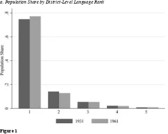
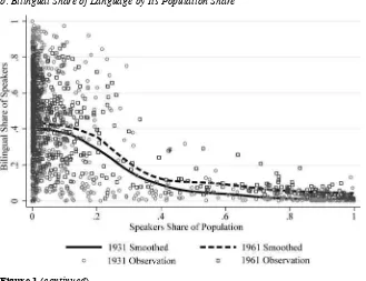
The fi rst panel of Figure 1 shows the population share of the top fi ve languages in each district. The typical district has a dominant language making up 75 percent of the population and several large secondary languages with population shares in 5 percent to 15 percent range. The growth in the share of the dominant languages mainly came at the expense of the language ranked second. The second panel of Figure 1 plots the bilingual share of speakers and speakers share of population for each district- language observation in the data for each year (N = 1,368). There is a great deal of variation in the bilingual share, particularly for the smaller languages at the left side of the fi gure. A fi t to the data from a kernel- weighted polynomial regression shows that on average the bilingual share rises roughly equally for all language sizes between 1931 and 1961.
Figure 1
Language Characteristics
Notes: Panel a. ranks each languages in a district from 1 to 5 by the number of speakers in 1931. Observations are weighted by the district population. N = 684.
IV.
Empirical Speci
fi
cation, OLS Estimates, and
Identi
fi
cation
In this section I present my main regression model, show some initial OLS estimates, and factors that may bias them. I then develop an instrumental vari-ables approach to address the biases.
The model measures the effect of industrial employment on bilingualism. Let Idt be the industrial share of total employment in district d at time t and Bldt be the share of mother- tongue speakers of language l in district d at time t that are bilingual. The panel structure allows me to eliminate language- district fi xed effect by differencing the data over time. My estimating equation is
(1) ∆Bld = α + β∆Id + sd + ∆εld
I do not aggregate the language data to the district level to allow for interactions. Most estimations will include a fi xed effect sd for the state to which a district be-longs to eliminate confounds from state industrial and education policy. Variation in industrial employment occurs at the district level, so I cluster the standard errors by b. Bilingual Share of Language by Its Population Share
Figure 1 (continued)
district. I weight the district- language observation by the number of speakers 1931 so that the coeffi cient β measures the effect of industrial share growth on the average individual.
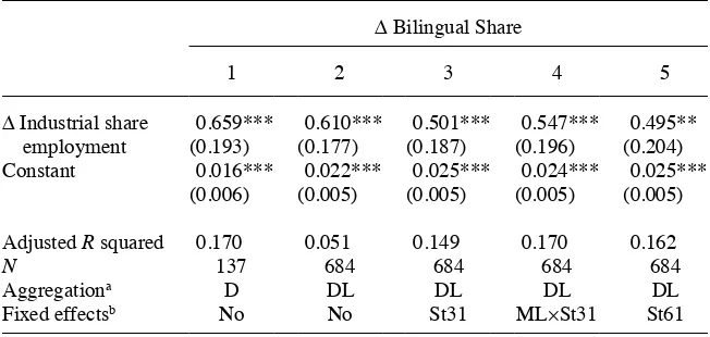
A. OLS Estimates
I begin the analysis with OLS estimates of Equation 1. For the sake of simplicity, I present an initial estimate with bilingualism aggregated to the district level (Table 2, Column 1). A change in the industrial share of employment of one percentage point is correlated with a 0.66- point increase in the share of the district population who are bilingual. The correlation is 0.61 in the full district- language data, which I will use for the remainder of the paper (Column 2). In interpreting the size of estimates, note that industrial employment share grew by an average 2.9 points between 1931 and 1961. If we assume a homogeneous effect, growth in the industrial share increased bilingual-ism by about 1.8 points. The overall bilingual share grew by 4.0 points, so industrial growth appears to be an important driver.
State governments undertook effort to improve education and to grow the manu-facturing sector, particularly after Indian independence in 1947. Column 3 introduces a fi xed effect for the state a district belonged to in 1931. This fi xed effect reduces the industrial share coeffi cient by about 18 percent to 0.50.
There were also many changes to the 1931 state boundaries over the panel that are related to language. Following popular agitations in the 1950s, the Government of India began to reorganize the states by grouping contiguous districts that shared a common Table 2
OLS Estimates
∆ Bilingual Share
1 2 3 4 5
∆ Industrial share 0.659*** 0.610*** 0.501*** 0.547*** 0.495** employment (0.193) (0.177) (0.187) (0.196) (0.204) Constant 0.016*** 0.022*** 0.025*** 0.024*** 0.025***
(0.006) (0.005) (0.005) (0.005) (0.005)
Adjusted R squared 0.170 0.051 0.149 0.170 0.162
N 137 684 684 684 684
Aggregationa D DL DL DL DL
Fixed effectsb No No St31 ML×St31 St61
Notes: Regressions are weighted by the average number of speakers of the district- language. Standard errors corrected for clustering at the district level. Stars indicate statistical signifi cance: * means p < 0.10, ** means
p < 0.05, and *** means p < 0.01.
a. D: Observation is a district; DL: Observation is a language within a district.
majority language into new states in order to create linguistically homogeneous states. The new organization may have affected both bilingualism and industrial growth. The reorganization placed regions of the 1931 states into different policy environments. For example, the Telugu- speaking region of Madras state was split off to form Andhra Pradesh in 1953. In 1956, the Telugu- speaking region of Hyderabad state was added to Andhra Pradesh. We can say that these two regions each had different policy environ-ments during the last years of the panel than other parts of their 1931 states.
To address this issue, I create a second fi xed effect that interacts the district majority language in 1931 with the 1931 state to allow for policy differences across regions due to the states reorganization. Column 4 shows an estimated effect of industrial growth of about 0.55 points, not much different from the 1931 state fi xed effects. I will use these fi xed effects in most specifi cations to follow. For the sake of compari-son, Column 5 shows that the industrial share coeffi cient is 0.50 when I include fi xed effects for the 1961 states. The estimates are also robust to a 1931 × 1961 state fi xed effects (not shown).
B. Sources of Bias
This section discusses biases in OLS estimates due to measurement error in the indus-trial share variable and correlation of the change in indusindus-trial share with both 1) omit-ted variables that affect bilingualism and 2) omitomit-ted endogenous variables, such as literacy, that are both affected by industrial growth and may themselves increase bilingualism.
The industrial work force variable suffers from measurement error due to a change in the way it was computed by the census. The 1931 Census categorized workers in each sector into one of three occupational categories: principal occupation, working dependents, or subsidiary occupation. Working dependents provided assistance to the worker in their job, such as the preparation of materials, though were not otherwise employed. Subsidiary workers had their principal occupation in another sector, which in the case of industry is overwhelmingly agriculture. Overall, 77 percent of industrial workers fell into the principal occupation category. In 1961, the census abandoned the three categories of workers, and counted only workers and nonworkers. I create my industrial employment variables using only the principal occupation data for 1931, which is most comparable to the 1961 categorization. Nevertheless, the change in the industrial share is measured with error, which would attenuate the OLS estimates.
In additional to industrial growth, urbanization, literacy, and income growth are also likely to encourage bilingualism. Urbanization brings populations into contact, creating both the demand for and opportunity to learn new languages. Literacy may be a complement or substitute for bilingualism, in both the acquisition of skill and its use. Income growth provides additional resources to invest in skills. These three processes are likely to be correlated with industrial employment growth and induce omitted variable bias.
Literacy and bilingualism can both be produced through attending school. Literacy can also be an important skill in the industrial workplace, particularly in the modern factory sector where rules and procedures are often written down. We would expect an upward bias of the OLS from the relationship of bilingualism and literacy. Similarly, urbanization brings people who speak different languages into contact, and is also driven by industrial growth, as factories tend to locate in cities. This also produces an upward bias.
The census provides data on literacy and urbanization. However, I cannot use them as controls in estimation because they are themselves outcomes of industrial growth. Literacy is of particular interest, as a related type of human capital, and I will treat it as an outcome in the analysis to follow.
C. Identifi cation
I address the threats to identifi cation from measurement error and time- varying omit-ted variables by constructing an instrumental variable for ∆Id. I take advantage of two aspects of Indian industry to provide a source of exogenous variation. The fi rst is persistence in the location of new industrial jobs. Districts with existing capacity in certain sectors have an advantage in capturing increased demand due to proximity to raw materials, economies associated with existing fi rm clusters, and other barriers to entry. Take steel production as an example. Proximity to coal and ore supplies confer cost advantages to steel mills. The second factor is the integration of Indian markets through an extensive railway network. Changes in demand for tradable industrial goods can be met by suppliers across the country.
My instrument uses variation in employment growth across 14 industrial sectors that comes from the interaction between national demand growth and the existing sectoral structure of industry at the district level. More concretely, the instrument is a prediction of the change in a district’s industrial share under the counterfactual as-sumption that each of its 14 sectors grew at the overall sectoral average. This type of instrument was pioneered by Bartik (1991) and Blanchard and Katz (1992), and has had several recent applications (Autor and Duggan 2003; Luttmer 2005; Card 2009; Lewis 2011). For example, Card (2009) and Lewis (2011) use the persistence in fl ows of migrants from particular countries to U.S. cities to form an instrument for changes in the skill mix of workers. My approach differs from this earlier work in using the predicted value from a regression rather than direct computation to produce the in-strument. This has the advantage of allowing me to exclude a district’s infl uence on overall sectoral growth when computing its predicted value.
Let μjd = (gjd / gWd) – 1 measure how much faster or slower subindustry j in dis-trict d is growing relative to the overall employment in d. Let yjd31 be the share of overall employment in district d in subindustry j in 1931. Then we can rewrite Equa-tion 2 as
(3) ∆Id= j
∑
μjdyjd31The relative growth rate μjd can be decomposed as μjd = μj + μ͂jd. The component μj is the average growth rate of employment in j relative to overall employment. The district- subindustry deviation from this average is μ͂jd. We then have
(4) ∆Id=
The fi rst term in Equation 4 is the component of the change in the industrial em-ployment share that refl ects whether a district’s initial complement of industries were relatively fast or slow growers on average. We can write the deviation as a residual and estimate the regression
(5) ∆Id= j
∑
δjyjd31+ζjdThe predicted value from this regression ∆Zd is just ∑joμj yjd31.
The predicted value ∆Zd will be a valid instrument if the exclusion restriction holds—subindustry employment shares and predicted values must be uncorrelated with time- varying unobservables. A concern immediately arises for those districts that have a large share of national employment in a particular subindustry. There were six districts that had more than 10 percent of national employment in at least one subin-dustry. The estimated coeffi cient δ̂j for the concentrated subindustries will be strongly infl uenced by the change in industrial employment in those districts and therefore potentially correlated with unobservables. A benefi t of using a regression rather than tabulated averages is that I can compute ∆Zd separately for each district d by 1) esti-mating Equation 5 on the districts ~d to compute δ̂j~d and then 2) making an out- of- sample prediction for district d.
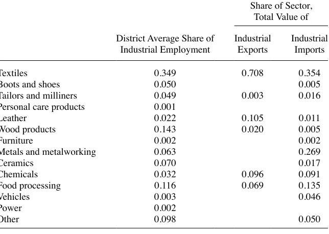
To create the instrument I collected district- level data on employment for 14 in-dustrial sectors in 1931. Table 3 shows summary statistics for the sectors. The largest sector is textiles, employing about one- third of all industrial workers. Wood products is the next largest industry, followed by food processing.
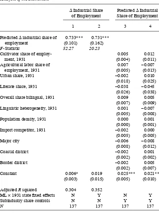
First- stage regressions are shown in Table 4. The instrument is strongly correlated with the actual change in the industrial share. The F- statistics of 52.27 on the bivariate correlation and 20.23 on the specifi cation with state fi xed effects imply that IV bias will be small. The coeffi cient on the instrument is 0.73, which implies that the IV estimate will not be sensitive to small violations of the exclusion restriction. I discuss this further below.
controlling for the subindustry shares. All of the coeffi cients are small and insignifi -cant. The 1931 characteristics are also jointly insignifi cant. I also provide some sensi-tivity tests for the exclusion restriction below.
V. Empirical Analysis
This section presents my estimates of the causal effect of industrial employment expansion on bilingualism. After discussing the basic results and sensi-tivity of the IV estimate, I explore the heterogeneity of the effect by how intensively a district was involved in trade, the particular second language learned, the size of the fi rst language, and the linguistic diversity of the district. Finally, I investigate the mechanism in more detail by comparing the effects of industrial growth on literacy and bilingualism, testing whether migration is an important source of bilinguals, and investigating assimilation. I conclude the section with an analysis of the affects of bilingualism on the evolution of a language community over time.
I present the main instrumental variables results in Table 5. Estimates are presented Table 3
Industrial Sectors in 1931
Share of Sector, Total Value of District Average Share of
Industrial Employment
Industrial Exports
Industrial Imports
Textiles 0.349 0.708 0.354
Boots and shoes 0.050 0.005
Tailors and milliners 0.049 0.003 0.016
Personal care products 0.001
Leather 0.022 0.105 0.011
Wood products 0.143 0.020 0.005
Furniture 0.002 0.002
Metals and metalworking 0.063 0.269
Ceramics 0.070 0.017
Chemicals 0.032 0.096 0.091
Food processing 0.116 0.069 0.135
Vehicles 0.003 0.046
Power 0.002
Other 0.098 0.050
Table 4
Analysis of the Instrument
∆ Industrial Share of Employment
Predicted ∆ Industrial Share of Employment
1 2 3 4
Predicted ∆ industrial share of 0.733*** 0.731***
employment (0.101) (0.162)
F- Statistic 52.27 20.23
Cultivator share of employ- 0.005 0.012
ment, 1931 (0.004) (0.011)
Agricultural labor share of 0.007 –0.007
employment, 1931 (0.005) (0.013)
Urban share, 1931 –0.002 0.010
(0.018) (0.025)
Literate share, 1931 –0.038 –0.045
(0.026) (0.038)
Overall share bilingual, 1931 0.009 0.005
(0.007) (0.009)
Linguistic heterogeneity, 1931 0.001 –0.007
(0.005) (0.008)
Population density, 1931 0.000 0.001
(0.000) (0.001)
Import competitor, 1931 –0.002 0.000
(0.005) (0.005)
Major city –0.006 –0.008
(0.008) (0.012)
Coastal district –0.002 0.001
(0.002) (0.002)
Border district –0.002 0.005
(0.002) (0.007)
Constant 0.006* 0.019 0.025*** 0.021**
(0.003) (0.015) (0.005) (0.010)
Adjusted R squared 0.304 0.352
ML × 1931 state fi xed effects N Y N Y
Subindustry share controls N N Y Y
N 137 137 137 137
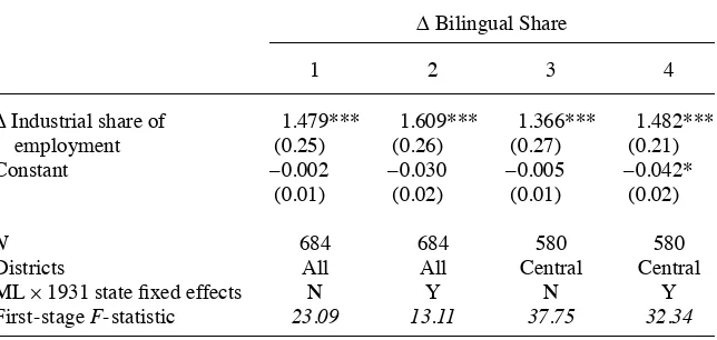
with and without state fi xed effects. The fi rst two columns show that a one- point increase in the industrial employment share produces a 1.5- point increase in the bi-lingual share. The estimate is large, both relative to the OLS and in an absolute sense. The estimated effect includes spillovers. For example, a new industrial job may lead to additional demand for transportation and commercial services.
Measurement error, as discussed in the previous section, is one reason why the IV estimate would be larger than the OLS. A second factor is that the IV procedure pro-duces an estimate of the local average treatment effect, or LATE (Imbens and Angrist 1994; Angrist and Pischke 2009). The IV estimator recovers a weighted average esti-mate of the causal response of each district- language to industrial growth, where the weights are proportional to the fi rst- stage impact on the district. Even if the OLS esti-mate were unbiased, to the extent that the responses are heterogenous across languages, the IV estimator can produce a different average estimate because it uses different weights.6
Recall that the instrument is an estimate of how national- level demand growth in subindustries would affect a district based on its 1931 structure. This variation will have a stronger effect on some districts than others. For goods that do not trade across districts, for example, national demand growth may not matter as much, and for industries where existing locations confer no advantage, the 1931 sectoral struc-ture may not matter much. The R2 for the
fi rst stage in Table 4, Column 1 is 0.31, Table 5
IV Estimates of Industrial Share Effects on Bilingualism
∆ Bilingual Share
1 2 3 4
∆ Industrial share of 1.479*** 1.609*** 1.366*** 1.482***
employment (0.25) (0.26) (0.27) (0.21)
Constant –0.002 –0.030 –0.005 –0.042*
(0.01) (0.02) (0.01) (0.02)
N 684 684 580 580
Districts All All Central Central
ML × 1931 state fi xed effects N Y N Y
First- stage F- statistic 23.09 13.11 37.75 32.34
Notes: Observations are at the district- language level and are weighted by the average number of speakers. Standard errors corrected for clustering at the district level. Stars indicate statistical signifi cance: * means
p < 0.10, ** means p < 0.05, and *** means p < 0.01.
6. As a concrete example, I can make a dummy variable that cuts my instrument at the mean and assign the value 1 to districts with above- mean values of the instrument and 0 to the others. This dummy has a strong
which means that much of the variation in industrial growth is not affected by the instrument.
We thus need to employ caution in comparing the LATE estimate to average changes in bilingualism and industrial growth. For example, if we take overall average industrial employment growth of 2.9 points and multiply it by the LATE of 1.6, we get an increase in bilingualism of 4.4 points, larger than the overall average. This compari-son is misleading because the average change in bilingualism and employment growth could be different from the local- average change corresponding to the estimate.
The correlation between industrial share growth and bilingualism is very strong both in the mountainous and linguistically diverse regions of north and east and in dis-tricts that border Pakistan, present- day Bangladesh, Nepal, and Burma. These regions saw the most dislocation during the partition of India in 1947, became sites of military garrisons, and also became more involved in border trade. I check the sensitivity of the estimates by excluding these districts in Columns 3 and 4, which show that the estimates are very close in the border and nonborder regions.
A. Trade and Import Competition
India increased import tariffs substantially through the 1920s, and they remained high until the end of my panel. The tariffs stimulated growth in import- competing industries. If national growth in industry is substantially driven by import substitu-tion, part of the difference between the OLS and IV estimates may refl ect the relative importance of bilingualism in tradable versus nontradable industrial goods.
I collected data on the value of India’s imports and exports of manufactured goods (India 1933b). I matched goods to the industrial sectors that produced them (for ex-ports) or that would produce them had they been made domestically (for imex-ports). Table 3 shows the shares of total export and import value assigned to each sector. Textiles dominate both imports and exports. Leather and chemicals are the second and third largest sources of export value, while metals and foods occupy those slots for imports.
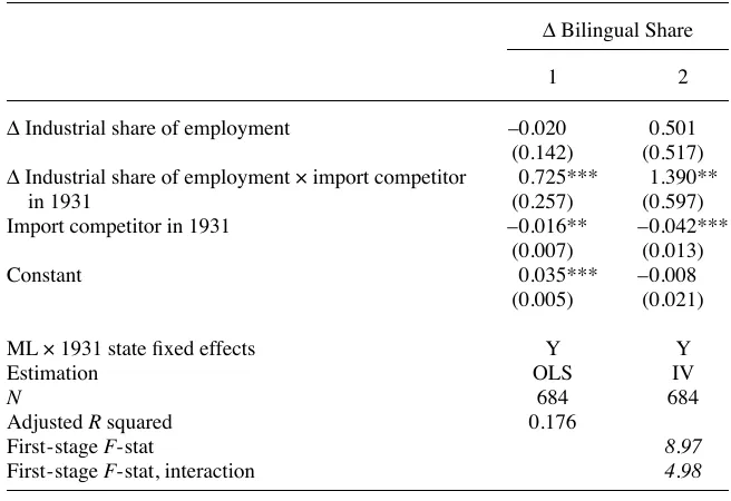
I used this data to construct an indicator of the degree to which each district’s manu-facturing employment was in sectors in which India was a net importer. For each district and sector, I calculate the share it contributes to national employment in the sector. I then assign the net import value of the sector as a whole to the districts using these shares. I sum this net import value within districts, which gives me a measure of how sensitive a district would be to changes in India’s trade policy. I create a dummy variable equal to one for those districts that have an above- median value of net im-ports. I call these above- median districts import competitors. The dummy variable tells us that a district’s manufacturing sectors overlapped relatively strongly with the goods of which India was a net importer. The industrial share increased by 4.3 points for import competitors and only 1.8 points for the others. The import- competing dis-tricts were more intensively involved in the production of textiles, processed foods, chemicals, vehicles, and power, and less intensively involved in wood, ceramics, leather, and tailoring.
nonimport competitors and 1.89 for import competitors. These estimates support the idea that bilingualism is particularly important in the production of tradable goods and that the instrument gives more weight to those districts.
B. Sensitivity of the IV Estimates
Another factor that might produce IV estimates much larger than OLS is a positive correlation between the instrument and the error term. This is a failure of the exclu-sion restriction. I will now explore how sensitive the IV estimates are to such positive correlations. If we write out the two IV stages explicitly as
(6) ∆Bld = α + β∆Id + γ∆Zd + ∆υld (7) ∆Id = θ + π∆Zd + ∆ϕld,
then the exclusion restriction amounts to the assumption that γ = 0.
It is easy to show that the bias is β̂ – β = γπ. Table 3 tells us that π̂ = 0.73, which means that the bias is approximately 1.36γ. A benefi t of having such a strong instrument is that the bias will be small even if the exclusion restriction holds only approximately. Table 6
Differential Effects by Import Competition
∆ Bilingual Share
1 2
∆ Industrial share of employment –0.020 0.501
(0.142) (0.517)
∆ Industrial share of employment × import competitor 0.725*** 1.390**
in 1931 (0.257) (0.597)
Import competitor in 1931 –0.016** –0.042***
(0.007) (0.013)
Constant 0.035*** –0.008
(0.005) (0.021)
ML × 1931 state fi xed effects Y Y
Estimation OLS IV
N 684 684
Adjusted R squared 0.176
First- stage F- stat 8.97
First- stage F- stat, interaction 4.98
Notes: Observations are at the district level and weighted by average district population. Standard errors corrected for clustering at the district level. Stars indicate statistical signifi cance: * means p < 0.10, ** means
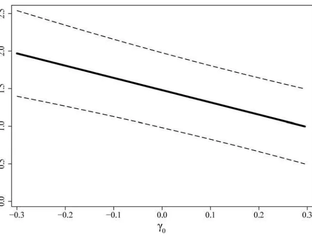
We can see how the IV estimates vary by choosing a set of fi xed values for γ, which I will call γ0, and then estimating
(8) ∆Bld – γ0∆Zd = α + β∆Id + ∆υld
By doing a separate estimation for each value γ = γ0 that is of interest, we can evaluate the sensitivity of the IV estimate of β (Conley, Hansen, and Rossi 2012).
Figure 2 plots the IV estimate and confi dence intervals for γ0∈[–0.3, 0.3]. The IV estimates are not very sensitive to even moderate amounts of bias. A correlation of ±0.1 yields estimates of 1.63 and 1.32. The endpoints of this interval represent a very substantial amount of bias, up to half as large as the reduced form OLS coeffi cient on industrial growth itself, and yet all are within the confi dence interval of the actual IV estimate.
C. Secondary Languages and Heterogeneous Districts
Industrial share growth had a greater impact on bilingualism for speakers of secondary languages (Table 7, Column 1). Because they comprise a small share of the population, Figure 2
Sensitivity of IV Estimates to the Exclusion Restriction
secondary language speakers have the greatest theoretical potential to expand the pool of others with whom they can communicate. This point can be formalized in a simple model. (See online appendix: http: // jhr.uwpress .org.)
My estimates show a one- point increase in industrial employment raises the likeli-hood of being bilingual for an average dominant language mother- tongue speaker by 1.3 points and for an average secondary language mother- tongue speaker by 2.1 points. The difference between these effects is positive with p = 0.11.
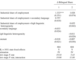
In more linguistically heterogeneous districts, impediments to communication will generally be higher, while the benefi ts of learning any particular second language will generally be smaller. The impact of growth in the industrial share in such districts in ambiguous. I divide districts into high and low linguistic heterogeneity groups by the median heterogeneity in 1931. The two groups of districts are similar in terms of initial levels and changes in industrialization, literacy, and urbanization, though we should keep in mind that linguistic heterogeneity may be correlated with unobservables. I estimate differential effects of industrial share growth for high heterogeneity districts Table 7
Differential Effects by Secondary Language and Heterogeneous Districts
∆ Bilingual Share
1 2
∆ Industrial share of employment 1.333*** 1.028
(0.351) (0.874)
∆ Industrial share of employment × secondary language 0.757 (0.610)
∆ Industrial share of employment × high linguistic 0.655
heterogeneity (0.842)
Secondary language –0.033
(0.024)
High linguistic heterogeneity –0.011
(0.029)
Constant –0.018 –0.007
(0.021) (0.036)
N 684 684
ML × 1931 state fi xed effects Y Y
Estimation IV IV
First- stage F- stat 19.54 5.43
First- stage F- stat, interaction 19.98 11.88
Notes: Observations are at the district- language level and are weighted by the average number of speakers. Standard errors corrected for clustering at the district level. Stars indicate statistical signifi cance: * means
in Column 2 of Table 7. The point estimates suggest a greater impact in heterogeneous districts, though the estimates are imprecise.
D. Choice of Second Languages
What languages did people learn as a result of industrial employment growth in India? English and Hindi are the major lingua francas of India. For speakers of uncommon languages in a locality, the local majority language would likely provide the greatest increase in the probability of being able to speak with the average person.
I have collected additional district- language level data from the 1961 census on the number of bilinguals in English and Hindi as well as bilinguals overall. The census did not tabulate data on the specifi c second language spoken at the district level in 1931 (or in any other census year). I therefore conduct the analysis in levels, estimating how the share of speakers of a district- language who are bilingual in English, Hindi, or another language is affected by industrial growth over the prior 30 years, controlling for the overall level of bilingualism for each district- language in 1931. This estimation includes state fi xed effects. It differs from the other specifi cations in this paper by not including district- language fi xed effects.
Table 8 shows IV estimates with interactions for minority languages. For speak-ers of the district dominant language, industrial growth had the strongest effect on learning Hindi, with a coeffi cient of 1.43, and smaller 0.88 effect on learning English. Learning other second languages was actually decreased by industrial growth by 0.49. In south India, Hindi has long been associated with north Indian dominance and is not widely used as a lingua franca. As we would expect, industrial growth leads predomi-nantly to English bilingualism in the south for dominant languages (regression not shown). Speakers of secondary languages had similar effects for all three categories: 0.95 for English, 0.39 for Hindi, and 0.78 for other. Outside of Hindi- majority areas, the dominant language will fall into the other category, which explains the large effect for secondary speakers.
These results relate quite directly to the evolving literature on the returns to English in the IT and business process outsourcing sector in the present day. They show that bilingualism in a lingua franca has been an economically important skill not only over the long run but also in the lower- skilled and much larger industrial sector.
E. Literacy
This section turns to the effect industrial employment expansion had on the invest-ment in literacy and makes comparisons with bilingualism. Literacy expanded from 9 percent to 27 percent of the population between 1931 and 1961. Recall that the standard of literacy used by the census was that a person be able to read and respond to a simple letter. The fact that only 8 percent of the Indian population had completed primary school in 1961 reminds us that learning to read does not require extensive instruction.
Column 1). This is very close in magnitude to the coeffi cient on bilingualism in the same specifi cation, which was 0.55. The expansion in literacy (18.1 points) was much larger than that of bilingualism (4.1 points), which makes industrial growth appear relatively less important as a driver of literacy growth. The IV estimate is 1.14, about twice as large as the OLS (Column 2). The difference refl ects the same set of factors discussed above for bilingualism. Because the same fi rst- stage is used in both cases, the sensitivity to the exclusion restriction is similar for this estimate.
I show how the effect on literacy varies by import competing status in Column 3. Literacy in import competing districts is more affected by industrial growth, but the difference is quite small: 1.17 versus 0.92 points. This difference was stronger for bi-lingualism: 1.89 versus 0.50. Demand for literacy was relatively similar across indus-tries, whereas bilingualism was more important in the import- competing ones. This Table 8
Industrial Share Growth and Bilingualism by Second Language in 1961
1961 Share of Speakers Who Were Bilingual in English
1
Hindi 2
Other 3
∆ Industrial share of employment 0.875*** 1.428*** –0.493**
(0.336) (0.399) (0.210)
∆ Industrial share of employment × 0.077 –1.034* 1.269**
secondary language (0.236) (0.577) (0.576)
Secondary language –0.004 0.026 0.046*
(0.007) (0.021) (0.025)
Share of speakers bilingual in 1931 –0.090 –0.240* 0.732***
(0.065) (0.140) (0.120)
Share bilingual in 1931 × secondary 0.080 0.272* –0.136
language (0.065) (0.148) (0.124)
Constant –0.011 –0.042* 0.016
(0.014) (0.023) (0.010)
N 682 567 684
State fi xed effects Y Y Y
Estimation IV IV IV
First- stage F- stat 10.43 10.43 10.43
First- stage F- stat, interaction 46.80 46.80 46.80
Notes: Observations are at the district- language level and are weighted by the average number of speakers. Columns 1 and 2 exclude mother tongue speakers of English and Hindi, respectively. Standard errors cor-rected for clustering at the district level. Stars indicate statistical signifi cance: * means p < 0.10, ** means
Clingingsmith
99
∆ Literate Share
∆ Bilinguals per Literate Person
1 2 3 4 5
∆ Industrial share of employment 0.538*** 1.138*** 0.923*** 14.810*** 13.113**
(0.126) (0.326) (0.298) (5.342) (5.275)
∆ Industrial share of employment 0.246
× Import competitor in 1931 (0.461)
Import competitor in 1931 –0.003***
(0.011)
Constant 0.138*** 0.107*** 0.109*** –1.370*** –0.819***
(0.018) (0.017) (0.015) (0.279) (0.265)
N 137 137 137 137 137
ML × 1931 state FE Y Y Y Y Y
Estimation OLS IV IV OLS IV
Adjusted R- squared 0.647 0.498 0.506 0.054 0.451
First- stage F- stat 10.19 6.13 10.19
First- stage F- stat, interaction 3.97
suggests that there are differences across sectors in the relative demand for literacy and bilingualism.
F. Bilingualism and Literacy
How much of the industrial share effect on bilingualism might be a consequence of increased literacy? Is it likely that, as both bilingualism and literacy can be outputs of a formal education, most of the unconditional effect of the industrial share on bilin-gualism actually operates through increasing literacy, so that bilinbilin-gualism is a kind of byproduct of literacy?
Bilingualism is certainly a stepping stone to literacy if one wishes to read a different language than one’s mother tongue. However, all languages in my data have scripts and written forms, so bilingualism wasn’t strictly necessary for literacy. Chaudhary (2010) reports that only 14 percent of literates knew English in 1931. Further, given the low level of primary completion in 1961 compared to the level of literacy and the fairly rudimentary literacy standard, it isn’t necessarily true that most people who became literate did so through schooling rather than a more informal arrangement. However, schooling was not offered in all languages in all places, and so some of those desiring education would have learned a second language to do so.
However, bilingualism and literacy do move together. The coeffi cient on the change in literacy regressed on change in bilingualism is 0.28. The correlation is even stron-ger, 0.52, if we look within policy environments by including state fi xed effects.7
Overall, literacy grew faster than bilingualism. The number of bilinguals per literate fell from 1.47 in 1931 to 0.55 in 1961. My unconditional estimates of the industrial share effect of bilingualism, 1.61, is higher than that on literacy, 1.14, suggest that industrial growth works against the trend. The fi nal two columns of Table 8 show that a one- point increase in the industrial share increased the number of bilinguals per literate by 13 points. At the mean change in the industrial share of 2.9 points, with the usual caveat about LATE, the IV estimate in Column 5 suggests industrial growth increased the ratio by 0.38 bilinguals per literate.
Rigorously estimating the effect of the industrial share on bilingualism conditional on literacy is more diffi cult. We would need an additional instrument for literacy. Even so, the fi rst stages of the conditional estimates would be different than the un-conditional ones, which implies that, following the logic of LATE, the un-conditional and unconditional estimates might not be strictly comparable.
I take the simpler approach of investigating how the IV estimate changes for fi xed values of the coeffi cient on literacy as a conditioning variable. In the spirit of the sensitivity test conducted above, consider the regression
(9) ∆Bld – θLld = α + β∆Id + sd + ∆εld,
where Lld is the change in the literate share of the population. How will the estimate of
β̂ change for different fi xed values θ0? If θ0 is positive, β̂ will fall.
I estimate Equation 9 for various θ0 and plot the results in Figure 3. Were the entire effect of industrial growth on bilingualism to actually come through literacy, we would need to have θ0 > 1.5. In other words, even if literacy and bilingualism were perfect
complements in production, there still would need to be substantial additional spill-overs from literacy into bilingualism to drive away the effect of industrial growth. If
θ = 1, we have β̂ = 0.48, and if it is the same size as the unconditional correlation with bilingualism, θ = 0.52, then β̂ = 1.02.
G. Learning, Migration, and Assimilation
Learning, migration, and assimilation are the most plausible channels through which a change in the industrial share would affect bilingualism. Human capital theory says people will learn a second language when the net benefi ts are high enough. These benefi ts may motivate bilinguals to move into a district where industrial employment is growing. The effect of the industrial growth could result in part from the sorting of bilinguals across districts. Industrial employment growth may also spur in- migration of monolinguals, which would also affect the bilingual share. Assimilation is also a mechanism through which the bilingual share may change. If parents decide to teach their children only their second language, the children become monolinguals in a dif-ferent mother tongue group from their parents.
In this section I will present evidence about the roles played by migration and as-Figure 3
Sensitivity of IV Estimates to the Conditional Effect of Literacy