Matthew Freedman is an assistant professor of economics at Cornell University. He thanks Len Burman, Jorge De la Roca, Andrew Hanson, Henry Overman, Emily Owens, Stuart Rosenthal, seminar participants at various institutions, and two anonymous referees for helpful comments. He also thanks the Texas Offi ce of the Governor and the Texas Comptroller of Public Accounts for assistance with the data used in this study. The research reported in this article used resources provided by Cornell University’s Social Science Gateway, which is funded through NSF Grant 0922005. The data used in this article can be obtained October 2013 through September 2016 from the author at 262 Ives Faculty Building, Cornell University, Ithaca, New York 14853, freedman@cornell.edu.
[Submitted January 2012; accepted May 2012]
SSN 022 166X E ISSN 1548 8004 8 2013 2 by the Board of Regents of the University of Wisconsin System T H E J O U R N A L O F H U M A N R E S O U R C E S • 48 • 2
Local Labor Markets
Matthew Freedman
A B S T R A C T
This paper uses a regression discontinuity design to examine the effects of geographically targeted business incentives on local labor markets. Unlike elsewhere in the United States, enterprise zone (EZ) designations in Texas are determined in part by a cutoff rule based on census block group poverty rates. Exploiting this discontinuity as a source of quasi- experimental variation in investment and hiring incentives across areas, I fi nd that EZ designation has a positive effect on resident employment, increasing opportunities mainly in lower- paying industries. While business sitings spurred by the program are more geographically diffuse, EZ designation is associated with increases in home values.
I. Introduction
many of its own place- based initiatives, it is all the more important to understand if and how these programs affect economic activity in targeted areas.
While EZs are often hailed by politicians as vital economic development tools, the evidence on their actual effects is decidedly mixed. Early work on EZ programs, which frequently used propensity score- matching techniques in an attempt to address omitted variable and selection problems, came to confl icting conclusions on the effects of zone designation on local labor markets (see, for example, Bondonio and Engberg 2000; O’Keefe 2004). However, more recent work that better accounts for unobserv-able differences among areas that could affect assignment to EZs and infl uence local labor market outcomes has also produced mixed results. For instance, Billings (2009) and Neumark and Kolko (2010) use narrow buffers outside EZs as control groups for EZs. While Billings (2009) documents positive employment effects, Neumark and Kolko (2010) fi nd no effects. However, though potentially mitigating bias owing to omitted variables, using areas geographically close to EZs as control groups could amplify bias due to spillovers.
Meanwhile, Busso, Gregory, and Kline (2011), who compare outcomes in census tracts that are designated federal Empowerment Zones to outcomes in tracts considered for but initially denied Empowerment Zone status, fi nd that zone designation increases employment.1 Using a double- difference estimation approach, Ham et al. (2011) also fi nd that state and federal zone programs have positive effects on neighborhood condi-tions and employment. Similarly, using a two- stage strategy to evaluate French EZs, Gobillon, Magnac, and Selod (2012) fi nd that designation reduces the duration of un-employment spells for workers in zones. In each of these studies, though, nonrandom selection of cities or neighborhoods into or out of treatment represents a major concern.
This paper adopts a new approach to evaluating the impact of EZs by taking ad-vantage of the unique structure of the Texas EZ Program. In contrast to most other states, where localities often must apply for EZ designations, Texas designates areas as EZs on a noncompetitive basis. In particular, any census block group that meets a minimum poverty criterion is automatically an EZ. This rule- based assignment of EZ status facilitates a regression discontinuity (RD) design in which I exploit the formula determining block group EZ designation as a source of quasi- experimental variation in investment and hiring incentives across geographic areas. My identifi cation strategy not only does not depend only on nearby areas as counterfactuals, but also circumvents omitted variable and selection problems that have plagued many past evaluations of place- based programs.
The Texas EZ Program creates explicit incentives to hire from, although not neces-sarily create jobs in, areas designated as EZs. Consistent with the program’s incentive structure, I fi nd using rich administrative data derived from unemployment insurance records that EZ designation increases resident employment in block groups with pov-erty rates near 20 percent by 1–2 percent per year. The employment effects are con-centrated in jobs paying less than $40,000 annually and are largely in the construction, manufacturing, retail trade, and wholesale trade industries. Estimates based on resident survey data corroborate these results and also point to measurable impacts of zone des-ignation on local property values. Further, while I cannot entirely rule out spillovers, EZs do not appear to be merely shifting jobs from nearby areas. Not surprisingly given
the structure of the program, which places fewer constraints on where fi rms locate than from which areas they hire, the effects on job creation in poor areas are less precisely estimated. The results are consistent with a more diffuse effect of the program on the locations of the new jobs in which residents of targeted regions are employed.
Focusing on one state’s EZ program allows me to isolate the outcomes most in line with its stated goals and to leverage particular institutional details to help identify the impacts on local labor markets. This would be more diffi cult with a broader sample given the variation across state and federal zone programs in the types of areas targeted, the types of incentives offered, and the generosity of those incentives. In part because of such variation, the results in this paper do not necessarily extend to all zone programs. Moreover, the RD design only permits me to identify the local average treatment effect of the program; that is, the results are only valid for a narrow group of census block groups with poverty rates near 20 percent. Designating much richer or much poorer neighborhoods as EZs would not necessarily have the same impacts I fi nd for the spe-cifi c group of communities I consider in this analysis. Nonetheless, my results shed new light on the effi cacy of place- based programs aimed at revitalizing blighted regions.
The paper is organized as follows. The next section provides an overview of Texas’ EZ Program. Section III discusses my strategy for identifying the impact of EZ desig-nation in Texas, which relies on a discontinuity generated by the formula the state uses to determine EZ status for census block groups. Section IV describes the data I use in the analysis. Section V presents the main results on the effects of EZs on resident and workplace employment as well as a series of robustness tests. I delve into the het-erogeneous effects of the program across different types of jobs in Section VI before considering possible spillovers in Section VII. Section VIII examines the impacts of EZ designation on other neighborhood conditions. Section IX concludes.
II. The Texas Enterprise Zone Program
A. Program Structure
First introduced in late 1980s, the Texas EZ Program is aimed at providing a means by which the state government and municipalities can reduce regulatory hurdles and provide certain incentives to encourage private investment and hiring in blighted ar-eas. Under the current program, which was created in 2003, participating businesses (known as Enterprise Projects) receive a combination of state and local benefi ts for up to fi ve years. These benefi ts take several forms. First, a single Enterprise Project can apply for state sales and use tax refunds of up to $1.25 million over fi ve years on qualifi ed expenditures on machinery and equipment, building materials, electricity and natural gas, and construction labor; the precise refund is tied to the amount of the capi-tal investment and the number of jobs created or retained at the site.2 Local communi-ties must also offer incentives to designated projects; these incentives may include tax abatement, utility rate reductions, public service expansion (for example, road improvements), tax increment fi nancing, expedited permitting, or other incentives.3
2. For the complete refund schedule, see http: // www.texaswideopenforbusiness.com.
In contrast to program rules in many other states, businesses in Texas need not necessarily locate in an EZ to receive benefi ts, nor does locating in an EZ guarantee that a business will receive benefi ts.4 To be eligible for benefi ts, a business located in an EZ must ensure that 25 percent of its new employees will meet economically dis-advantaged or EZ residence requirements.5 A business located outside an EZ is eligible to receive benefi ts if it commits that 35 percent or more of its new employees will meet economically disadvantaged or EZ residence requirements. Therefore, more so than the number of jobs that exist in distressed areas, the program might be expected to increase the number of jobs held by the residents of those areas. Due in part to data limitations, past research has typically only examined one or the other, either using employer- side data on the location of jobs (see, for example, Bondonio and Engberg 2000; O’Keefe 2004) or resident- side information on employment or unemployment (see, for example, Elvery 2009; Gobillon, Magnac, and Selod 2012).6
Meanwhile, locating in or hiring from an EZ does not ensure a business will receive benefi ts. The local jurisdiction must nominate businesses for Enterprise Project des-ignations. Nominations are reviewed by the State Offi ce of Economic Development, which makes a fi nal determination about awards. Legislation limits the number of designations to 105 per biennium.7
The costs of the program are diffi cult to calculate, in part because the burden is shared by state and local governments and in part because different localities supple-ment the state’s incentives with different (and often project- specifi c) benefi ts. The Texas Comptroller of Public Accounts (CPA) estimates that the program cost the state alone $33.6 million during fi scal years 2008 and 2009; during that period, businesses receiving refunds pledged $5.7 billion in capital investment and over 13,000 new jobs (Texas CPA 2010). However, this does not immediately imply that the program is cost- effective; not only do the CPA’s fi gures not take into account the cost of benefi ts offered by localities, but much of that investment and job creation may have occurred in the absence of the program. The results of this paper speak to the extent of crowd- out of unsubsidized private- sector investment associated with Texas’ EZ Program.8
fees, and one- stop permitting. Houston offers property tax abatements and a small business revolving loan fund.
4. For example, in California, which Elvery (2009) and Neumark and Kolko (2010) consider in their analy-ses, businesses are eligible for benefi ts only if they are located in an EZ.
5. An economically disadvantaged person is defi ned as one who (a) was unemployed for at least three months before obtaining employment with a qualifi ed business, (b) receives public assistance benefi ts, (c) has a physical or mental disability, (d) is homeless, (e) is a foster child, (f ) is on parole or was recently released from a state correctional facility, or (g) is an individual whose family income meets the low- or moderate- income limits under the Section 8 program. To the extent that verifying economically disadvantaged status is more diffi cult than verifying residency, fi rms may have a preference for the latter. In any case, if Enterprise Projects hire economically disadvantaged persons as opposed to EZ residents, it will attenuate the effects of the state’s program on EZ resident employment.
6. Exceptions include Ham et al. (2011) and Busso, Gregory, and Kline (2011).
7. While they have no discretion over which areas are designated EZs, local offi cials have discretion over which projects they nominate and state offi cials can turn down applications. The state does not make informa-tion on failed applicainforma-tions available, but there is reason to believe that many are turned down because they were too late to apply during the biennium (all 105 designations had already been awarded).
B. EZ Designations
Since the program was amended in 2003, EZs in Texas have been designated accord-ing to a noncompetitive, rule- based assignment scheme.9 In particular, any census block group (as defi ned by the most recent decennial census) in which 20 percent or more of the residents have income below the federal poverty level is automatically designated an EZ. Further, any area designated by the federal government as an Em-powerment Zone, Renewal Community, or Enterprise Community is also designated a state EZ. Another amendment in 2005 stipulated that any county in the state in which the poverty rate exceeds 15.4 percent, at least 25.4 percent of the adult population does not hold a high school diploma (or equivalent), and the unemployment rate has remained above 4.9 percent for fi ve consecutive years is automatically designated an EZ.
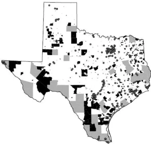
The shaded areas in Figure 1 represent the Texas EZs as of 2010.10 Of the 254 counties in the state, 34 were designated EZs based on county poverty rates, adult education rates, and unemployment rates. Meanwhile, 16 tracts covering parts of ten counties were designated state EZs by virtue of being federal Empowerment Zones or Renewal Communities (EZ / RCs).11 Altogether, those 34 counties and 16 tracts en-compass 1,465 (or 10.1 percent) of the 14,463 block groups in Texas. Of the remaining 12,998 block groups in the state, 3,598 (or 27.7 percent) of the block groups are EZs as a result of having a poverty rate of at least 20 percent. For the purposes of identi-fi cation, I focus on this latter group of block groups in the main analysis, although in robustness tests I take into account the overlap in programs. Notably, while most dis-tressed counties and federal EZ / RCs are concentrated along the border with Mexico, EZs designated on the basis of block group poverty rates are scattered throughout the state.12
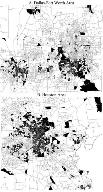
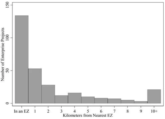
In addition to showing EZs in Texas, Figure 1 plots the locations of the roughly 300 Enterprise Projects that received awards between September 2003 and September 2010.13 Figure 2 zooms in on select urban areas in the state, including Dallas- Fort Worth and Houston.14 These fi gures make clear not only how physically small EZs in Texas can be, but also how Enterprise Projects tend to be near, but not necessarily in, EZs. Indeed, as Figure 3 shows, only 45 percent of the Enterprise Projects that could
9. Prior to 2003, EZs in Texas were required to be areas “of pervasive poverty, unemployment, and economic distress” and to be between one and ten square miles in size (see Texas State Government Code, Title 10, Subtitle G, Chapter 2303). Similar to most other states’ current programs, areas also had to be nominated by an ordinance or order adopted by a locality.
10. 2000 Decennial Census data were used to determine the eligibility of counties and block groups for EZ status from the start of the program through the present. The maps also refl ect 2000 Census geographic boundaries.
11. The tax benefi ts of federal Enterprise Communities expired in 2004.
12. One challenge that arises in determining the effects of EZs in many states is that EZ boundaries do not conform to standard census or postal boundaries for which one can obtain accurate measures of outcomes of interest (Elvery 2009). If some areas are misclassifi ed as EZs and others are misclassifi ed as controls as a result of the aggregation or manipulation of data to construct consistent geographic regions, it will tend to bias one toward fi nding no effect of EZs. After 2003 in Texas, this does not pose a problem, as all EZs in the state conform to FIPS codes.
13. 297 of the 320 business that received Enterprise Project designations between September 2003 and September 2010 could be precisely geocoded and appear on the map.
be geocoded were located in an area designated as an EZ between 2003 and 2010; the remainder were located outside EZs but received awards by pledging to hire at least 35 percent of their workforce from a disadvantaged group or from an EZ. Likely as a result of this requirement, 85 percent of Enterprise Projects were located within at least fi ve kilometers of an EZ. Over 99 percent of Enterprise Projects were located within 20 kilometers of an EZ.
III. Empirical Strategy
A. Model
This paper aims to identify the effects of EZ designation on local labor markets. I conduct the analysis at the level of census block group, which are geographies larger than a city block but smaller than a census tract. In Texas, block groups had a median population of 1,180 and a median area of 1.2 square kilometers in 2000.
Figure 1
Texas Enterprise Zones and Enterprise Projects
Figure 2
Enterprise Zones and Enterprise Projects in Selected Texas Cities
Following Chay and Greenstone (2005), Baum- Snow and Marion (2009), and Freedman (2012), I am interested in estimating β1 in the following equation:
(1) ∆yi = β0+β1EZi+ XiΩ+ εi
In Equation 1, yi is the outcome of interest for block group i, EZi is a dummy for whether i is an enterprise zone, and Xi is a set of baseline (year 2000) characteristics of i. Simply estimating Equation 1 on all block groups will likely yield inconsistent estimates of β1 given that unobserved and unmeasured local characteristics might be correlated with EZ status and independently affect the outcome of interest. If localities must apply for EZ designation (as they must do in many states), those localities that apply are likely to be different in unmeasurable ways than localities that do not apply. This selection problem has hampered past research on EZs.
Since September 2003, EZs have been designated in Texas according to a noncom-petitive, rule- based process in which local economic conditions determine EZ status. While this overcomes the selection problem associated with differences across areas related to the propensity to apply for EZ designations, there are still potential omitted variables at the block group level that could bias estimates of the effects of EZ status on local labor market outcomes. The decision of a business to invest in or hire from a particular place is likely to be infl uenced by local characteristics as well as expecta-tions about the future prospects of the area, each of which may not be fully captured in Xi and also might affect ∆yi. To the extent that we cannot control for such factors, the error term εi will be correlated with EZi, which in turn will bias estimates of β1.
Figure 3
Spatial Distribution of Enterprise Projects
To address this problem, I adopt an RD design that takes advantage of the rule determining EZ status. The approach in this paper builds on recent work exploiting the formula structure of various placed- based programs on neighborhoods (Baum- Snow and Marion 2009; Freedman and Owens 2011). In an RD framework, whether an observed covariate (the forcing variable) lies on either side of a fi xed cutoff value at least partly determines treatment.15 In Texas, outside of distressed counties and federal EZ / RCs, a block group’s poverty rate determines EZ status. Specifi cally, block groups with poverty rates of 20 percent or greater are EZs, while block groups with poverty rates less than 20 percent are not. Thus, for the subset of block groups that I consider in the main analysis, the discontinuity is “sharp” in the sense that no block groups with poverty rates below 20 percent qualify as EZs and all block groups with poverty rates above 20 percent qualify as EZs.16
The critical assumption behind my econometric approach is that block groups in a suffi ciently narrow window around the 20 percent poverty rate threshold are similar along observable as well as unobservable dimensions. More specifi cally, covariates besides EZ status that might affect the outcomes of interest cannot change discontinu-ously at the poverty rate threshold for EZ designation. If this is true, and if there is no sorting around the threshold, then for a population of block groups near the 20 percent poverty rate threshold, EZ designation is assigned essentially at random. In the next section and in Section IV.C, I argue and provide evidence that the preconditions for an RD design hold and that in turn, we can interpret any discontinuity in the conditional distribution of outcomes as a causal effect of EZ designation.
Following much of the literature on EZ programs, I examine the reduced form re-lationship between zone status and local labor market outcomes.17 The equation of interest is therefore
(2) ∆yi = γ0+γ1EZi+ f(pi)+ XiΨ+ui,
where pi is the poverty rate of block group i and f is a control function. I use a variety of specifi cations for f, including various polynomial specifi cations (quadratic, cubic, and quartic) in which the polynomial coeffi cients are allowed to differ above and be-low the cutoff.18 As I show in the results, the estimates vary only slightly with different specifi cations of the control function. Moreover, as I show in the results and as would
15. For a detailed discussion of RD designs, see Lee and Lemieux (2010).
16. In principle, one also could exploit the cutoffs for designation as a distressed county. However, there are only 254 counties in Texas, and many fewer close to the poverty, education, or unemployment thresholds for distressed county designation. In Section V.D, I include distressed counties and federal EZ / RCs as a robustness check.
17. If one considers an area treated if an Enterprise Project hires from or locates in that area, the coeffi cient on EZ refl ects an intent to treat. While I observe location for most Enterprise Projects, I do not have informa-tion on where Enterprise Project employees reside. Also, the intent to treat is arguably the outcome of interest from a policy perspective. Firms may locate in or near EZs in hopes of benefi tting from the program even if they ultimately do not. People may also move to EZs in hopes of benefi tting from the incentives businesses have to hire from those areas. Thus, the overall impact on neighborhoods of EZ designation, over which offi -cials also have more control than where Enterprise Projects invest, is of substantial policy import. 18. Specifi cally, I use control functions that take the following general form:
f(pi) = [φ1k(pi−0.2)k
be expected if the identifi cation strategy outlined here is valid, including controls in X
does not affect the results substantively.
B. Identifi cation
The main identifying assumption underlying the RD design employed in this paper is that unobservable determinants of ∆yi do not differ among census block groups within a narrow window around the poverty rate cutoff. One possible threat to this assumption is that sorting occurred among block groups around the threshold. While self- selection into treatment is a problem in the analysis of state EZs in most of the over 40 states that currently have zone programs, it is highly unlikely that such sorting occurred in the case of the Texas EZ Program. Designations for block groups outside distressed counties and federal EZ / RCs are determined strictly according to the pov-erty rate published in the most recent decennial census. Even if communities antici-pated the formula structure of the Texas EZ Program, it is unlikely that they would be able to manipulate the census results. Indeed, the sampling variability associated with the one- in- six sample drawn for the long- form 2000 Decennial Census, as well as im-putation and confi dentiality protection procedures conducted by the Census, add noise to the data that ensures local offi cials could not have perfect control over the value of the forcing variable for any given block group. As further checks on the assumption that no sorting occurred around the threshold that might invalidate the proposed RD design, in Section IV.C, I provide descriptive evidence and formally test that there is no discontinuity in the distribution of the forcing variable at the cutoff and show that observable baseline covariates evolve smoothly through the threshold.
Importantly, the RD estimates represent a weighted average of the effects of EZ designation for the subpopulation of neighborhoods near the cutoff, where the weights are proportional to the ex- ante likelihood of having a poverty rate near the threshold. The effects of EZ designation are unlikely to be the same in very high or very low income areas with poverty rates far from the cutoff. In other words, Equation 2 identi-fi es a local average treatment effect that may not be equal to the average treatment effect for the entire population of block groups. Nonetheless, estimates of the local average treatment effect are of substantial policy import. While an important dimen-sion over which state and federal zone programs differ is the criteria used to determine whether areas are suffi ciently “poor” to warrant designation, nearly all programs focus on low- income communities, and often communities with poverty rates not far from 20 percent.19
IV. Data
A. Sources
The data used in this analysis come from several sources. The fi rst is the Economic Development and Tourism division of the Texas Offi ce of the Governor, which pub-lishes on its website a list of EZs in the state that qualify on the block group poverty
rate criterion or as distressed counties.20 I combined these data with information on the location of federal EZ / RCs, which is published on the Department of Housing and Urban Development’s website. This left me with a data set encompassing all EZs in Texas.
Baseline resident characteristics of block groups were extracted from the 2000 De-cennial Census. These data include a host of demographic characteristics, including in-formation on total population, racial and ethnic composition, gender composition, the age distribution, the use of languages other than English (mainly Spanish in Texas), shares with U.S. citizenship, educational attainment levels, household and family in-come, unemployment rates, labor force participation rates, household mobility, and poverty rates. The data also include a number of housing- related variables, including total housing units, share vacant, share occupied, share owner occupied, share rented, median age of units, and median house value.
In order to examine the effects of the EZ Program on local labor markets over the 2000s, I obtained administrative data on resident and workplace employment by block group and year between 2002 and 2009 from the Longitudinal Employer- Household Dynamics (LEHD) Program at the U.S. Census Bureau.21 These data, which are de-rived from state unemployment insurance records, capture approximately 98 percent of private sector employment in the United States. Resident employment in a block group represents the number of residents in that block group who hold jobs (regardless of where those jobs are located). Workplace employment in a block group represents all jobs that are located in that block group (regardless of where the workers who hold those jobs reside). For both resident and workplace employment, these data contain job counts as well as the number of jobs in each of three pay categories (jobs paying less than $15,000 annually, jobs paying between $15,000 and $39,999 annually, and jobs paying $40,000 or more annually). Additionally, the data contain the number of resident and workplace jobs in each major industry (at the two- digit NAICS level). As outcome variables, I use the average annual change in log employment (either resident or workplace) in a block group.22 State sales and use tax refunds fl ow to Enterprise Projects on an annual basis. Also, average annual changes are more easily interpre-table than are changes over seven years (between 2002 and 2009).23
Due to their comprehensiveness, fi ne geographic resolution, and information on both resident and workplace employment, the LEHD data are well suited to study how EZ designations affect local labor markets. However, they have several drawbacks. First, they do not contain information on hours worked, so calculating hourly wages
20. The Economic Development and Tourism division of the Texas Offi ce of the Governor also provided me with a list of Enterprise Projects, or businesses that have received incentives through the state’s EZ program. 21. These data are derived from the LEHD Program’s OnTheMap program, which provides annual cross- sectional information on jobs at detailed geographies. I include in the sample all jobs, regardless of whether they are primary or secondary jobs. Restricting the sample to primary jobs, or the job for each person that contributes the most to his / her earnings each year, has little effect on the results.
22. I add one to both resident and workplace employment to avoid taking the log of zero. As less than 3 percent of observations have zero resident employment, workplace employment, or both, instead excluding observations with zero employment has little effect on the main results.
is not possible. Second, the earnings thresholds are not adjusted for infl ation each year, and hence there is a gradually declining fraction of jobs in the low- earnings bin and a gradually increasing fraction of jobs in the high- earnings bin. In the empirical analysis, I test whether EZs experienced differentially large or small changes in each type of job. Finally, for confi dentiality reasons, LEHD infuses noise into the resident employment data by synthesizing it from the true data in a method similar to data swapping (Andersson et al. 2008).24 This will tend to add measurement error to the dependent variables that should only be problematic to the extent that it is correlated with EZ designation.
Both as a robustness check on the resident employment results based on the LEHD data and in order to examine the impacts of Texas’ EZ program on other neighbor-hood conditions, I take advantage of recently released small- area estimates from the 2005–2009 American Community Survey (ACS). These estimates refl ect survey in-formation collected between January 1, 2005 and December 31, 2009, and hence the data capture average neighborhood characteristics over the entire fi ve- year period.25 The neighborhood outcomes of interest, including resident employment, population, poverty rates, median household income, median house values, and vacancy rates, are measured as changes between the 2000 Decennial Census and the 2005–2009 ACS. Notably, to the extent that the impact of EZ designation took time to affect neighbor-hoods, the estimated effects using the ACS will be attenuated.
B. Sample
In order to cleanly identify the effect of EZ designation on local labor market out-comes, I limit attention to the subset of Texas block groups that were not designated a distressed county or a federal EZ / RC at any point during the sample period. Dropping these block groups left me with 11,943 block groups. Of these, 11,692 had valid infor-mation for all the socioeconomic and housing variables in the 2000 Decennial Census.
For the RD assumptions to be valid, a suffi ciently narrow window around the rel-evant threshold must be used to ensure that observations on either side of the cutoff are similar along both observable and unobservable dimensions. While the latter cannot be verifi ed conclusively, the former can be. In the main analysis, I limit attention to census block groups with poverty rates (based on 2000 Decennial data) of between 18 percent and 22 percent (inclusive). The fi nal sample that has all requisite vari-ables available and that are outside distressed counties or federal EZ / RCs is 995 block groups. As robustness checks, I consider alternative windows around the 20 percent poverty rate threshold as well as placebo cutoffs.
24. Prior to 2006, LEHD suppressed information for blocks where the number of workers residing in the block was fewer than fi ve or where the number of different blocks where resident workers were employed was fewer than three. In rural areas in particular, this tended to bias downward aggregate estimates of resident employment. This will affect my estimates only to the extent that the error generated by cell suppression is correlated with EZ designation. Estimates based on only densely populated areas are qualitatively and quantitatively similar to the main results.
C. Descriptive Statistics
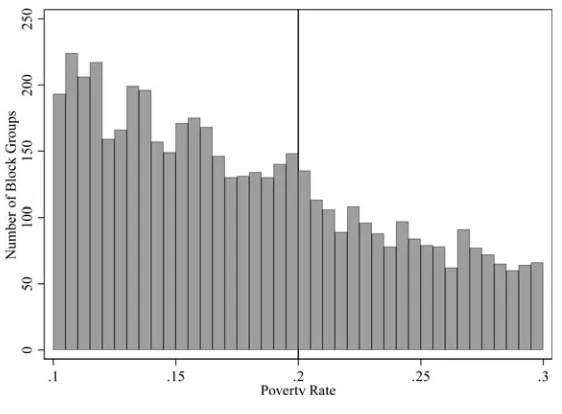
In Figure 4, I present a histogram showing the number of block groups in each half percentage point bin of the poverty rate in a 20 percentage point window around the 20 percent cutoff that determines EZ status for block groups in Texas. While fewer block groups have poverty rates close to 30 percent than poverty rates close to 10 percent, there is no indication of a discontinuity in the distribution of the forcing variable at the cutoff. A McCrary (2008) test confi rms there is no statistically signifi cant jump in the density function at 20 percent. This is consistent with a lack of any manipulation in the value of the poverty rate that might undermine the RD design.26
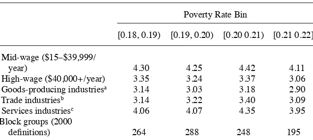
Table 1 presents descriptive statistics for census block groups in the main sample. In Panel A, average values for the baseline (year 2000) demographic and housing vari-ables are presented in one percentage point bins of the forcing variable on either side of the 20 percent threshold. Panel B shows 2002 resident and workplace employment information from the LEHD data in bins on either side of the cutoff, including fi gures broken out by earnings and broad industry.
There is little evidence that the covariates are anything but smooth through the cutoff.27 In fact, none of the differences in baseline demographic and housing
charac-26. The lack of any discontinuity in the forcing variable or the other baseline characteristics also indicates that there were no preexisting place- based programs that used the same cutoff whose impacts might obscure the effect of EZ designation on the outcomes of interest.
27. Building 2000- boundary block groups from 1990 blocks, I also checked for differential trends between 1990 and 2000 on either side of the threshold in population, share black, share Hispanic, share under age 30,
Figure 4
Density of the Forcing Variable
Table 1
Descriptive Statistics
Poverty Rate Bin
[0.18, 0.19) [0.19, 0.20) [0.20 0.21) [0.21 0.22]
A. Demographic and housing characteristics (2000 Decennial Census)
Log population 7.08 7.06 7.07 7.05
Share Black 0.15 0.18 0.16 0.17
Share Hispanic 0.32 0.37 0.37 0.42
Share male 0.50 0.49 0.50 0.50
Share younger than 30 0.46 0.47 0.47 0.48
Share age 65+ 0.12 0.12 0.11 0.11
Share households speak
Spanish 0.28 0.30 0.32 0.36
Share foreign born 0.14 0.15 0.17 0.17
Share same house as 5 years
ago 0.51 0.52 0.50 0.50
Share only high school
degree 0.29 0.28 0.28 0.28
Share some college 0.21 0.20 0.19 0.19
Share college degree 0.18 0.17 0.17 0.16
Unemployment rate 0.07 0.08 0.08 0.08
Labor force participation rate 0.61 0.60 0.61 0.59
Log household income 10.37 10.33 10.32 10.28
Log number of housing units 6.16 6.15 6.15 6.09
Share of homes vacant 0.10 0.10 0.10 0.09
Share of homes owner
oc-cupied 0.61 0.59 0.57 0.57
Log house value 10.91 10.87 10.88 10.86
Median house age 31.69 34.24 32.79 34.68
B. Employment characteristics (2002 LEHD)
Log resident employment 6.14 6.15 6.13 6.11
Low- wage (<$15,000 / year) 5.04 5.08 5.05 5.05 Mid- wage ($15–$39,999 /
year) 5.36 5.38 5.36 5.35
High- wage ($40,000+ / year) 4.44 4.37 4.38 4.27 Goods- producing industriesa 4.62 4.58 4.60 4.57
Trade industriesb 4.56 4.54 4.53 4.53
Services industriesc 5.48 5.52 5.48 5.47
Log workplace employment 5.16 5.09 5.28 4.94
Low- wage (<$15,000 / year) 4.10 4.12 4.31 4.02
teristics among block groups in the [0.19, 0.20) bin and the [0.20, 0.21) bin are statisti-cally signifi cant at the 5 percent level.28 Consistent with the density test of the forcing variable itself, tests of the null hypothesis of continuity of the density of each of the covariates, as well as that of the initial (year 2002) values of the outcome variables, against the alternative of a jump in the density suggest that there is no sorting around the threshold.29
V. Results
A. Main Results
In this section, I present results for my preferred sample, which consists of all block groups in Texas with poverty rates within a four percentage point window around the 20 percent threshold determining EZ status and excluding areas in distressed counties or federal EZ / RCs. In subsequent sections, I perform a variety of robustness tests to
share age 65 or over, number of housing units, share vacant, share owner- occupied, and median house values. There are no statistically signifi cant differences across the threshold in these trends, and the main regression results are robust to their inclusion as additional controls. Results are available upon request.
28. Differences across the threshold in only two covariates (the share of the population that is male and the share with some college) are signifi cant at the 10 percent level.
29. A chi- squared test based on a seemingly unrelated regression in which each equation is for a separate baseline covariate cannot reject the null that all the discontinuity gaps are jointly equal to zero. Graphical evi-dence of the lack of any discontinuities in baseline covariates at the threshold is also available upon request.
Table 1 (continued)
Poverty Rate Bin
[0.18, 0.19) [0.19, 0.20) [0.20 0.21) [0.21 0.22]
Mid- wage ($15–$39,999 /
year) 4.30 4.25 4.42 4.11
High- wage ($40,000+ / year) 3.35 3.24 3.37 3.06 Goods- producing industriesa 3.14 3.03 3.18 2.90
Trade industriesb 3.14 3.22 3.40 3.09
Services industriesc 4.06 4.07 4.35 3.95
Block groups (2000
defi nitions) 264 288 248 195
Note: Includes block groups in Texas that are not in distressed counties or federal EC / RZs and that are not missing 2000 Decennial Census information.
a. Goods- producing industries include agriculture, mining, utilities, construction, and manufacturing indus-tries.
b. Trade industries include wholesale trade, retail trade, and transportation and warehousing.
ensure that the results are not sensitive to the particular sample and specifi cations chosen.
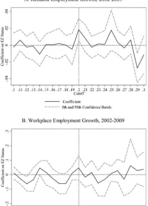
First, I show graphical evidence of differences in resident and workplace employ-ment growth across EZ and non- EZ block groups near the 20 percent threshold. Panel A of Figure 5 shows the average annual change in log resident employment within 0.1 percentage point bins in a four percentage point window around the 20 percent pov-erty rate threshold, while Panel B shows the average annual change in log workplace employment. In each case, there appears to be a discontinuity at the 20 percent cutoff, with higher employment growth above the threshold (in block groups that are EZs) than below the threshold (in block groups that are not EZs).
Corresponding regression estimates appear in Panels A and B of Table 2. Each en-try in the table is from a separate regression, where for different control functions (quadratic, cubic, and quartic), I present estimates based on regressions that include the control function alone (Columns 1, 4, and 7); the control function plus the demo-graphic and housing controls listed in Table 1 (Columns 2, 5, and 8); and the control function, demographic and housing controls, and county dummies (Columns 3, 6, and 9). The standard errors are adjusted for heteroskedasticity and clusters at the county level, which may overstate the standard errors somewhat by allowing for a fairly gen-eral covariance structure in which observations are assumed to be independent across counties but not necessarily within counties.30
Panel A of Table 2 indicates that, regardless of the form chosen for the control func-tion and which controls are included in the regression, the average annual difference in log resident employment is consistently 1–2 percent greater in areas just qualifying as EZs relative to similar areas that barely fail to qualify as EZs. The coeffi cient estimates are all statistically signifi cant at least at the 10 percent level, and most are signifi cant at the 5 percent level. Additional controls not only have little impact on the estimates, but also have little effect on their precision. The estimates imply an increase on average of 5–6 resident jobs per designated block group per year, or about 35–42 resident jobs over the time horizon under consideration.31
Turning to Panel B of Table 2, the estimates for the impact of EZ designation on workplace employment are slightly larger at 3–5 percent. However, the estimates are much less precise, likely a refl ection of the fact that the Texas EZ Program, while mak-ing locatmak-ing in EZs more desirable by lowermak-ing the share of employees that must be disadvantaged or from an EZ, does not require that businesses locate in EZs to receive EZ benefi ts. Hence, as Figures 1–3 hint, while some Enterprise Projects contribute directly to job creation in EZs, many contribute to job creation elsewhere (including in nearby non- EZ block groups). As a result, job creation spurred by the program is more geographically diffuse than are increases in resident job- holding, and the results are not defi nitive as to whether EZ status is associated with higher workplace employ-ment.
30. Of the 254 counties in Texas, 137 are represented in the regressions that include block groups with poverty rates between 0.18 and 0.22. Clustering at the level of census tract, of which there are 822 in the main sample, has little effect on the standard errors.
Figure 5
Resident and Workplace Employment Growth at the Poverty Rate Threshold for EZ Designation
T
he
J
ourna
l of H
um
an Re
sourc
es
Table 2
RD Estimates for Resident and Workplace Employment—Average Annual Change in Log Employment, 2002–2009
(1) (2) (3) (4) (5) (6) (7) (8) (9)
Panel A: Resident employment
Enterprise Zone dummy 0.011** 0.009* 0.011** 0.014* 0.013* 0.019*** 0.021** 0.019** 0.022*** [0.005] [0.005] [0.005] [0.008] [0.008] [0.007] [0.010] [0.010] [0.008]
Panel B: Workplace employment
Enterprise Zone dummy 0.045* 0.040 0.045 0.032 0.030 0.047 0.051 0.050 0.078 [0.025] [0.028] [0.033] [0.033] [0.033] [0.042] [0.046] [0.045] [0.058]
Quadratic in poverty rate Y Y Y
Cubic in poverty rate Y Y Y
Quartic in poverty rate Y Y Y
Demographic and housing controls Y Y Y Y Y Y
County dummies Y Y Y
Observations 995 995 995 995 995 995 995 995 995
B. Placebo Estimates
To verify that any observed jumps are in fact being driven by the EZ designation, I conduct a placebo exercise using a series of alternative thresholds. The results of this robustness check appear in Figure 6, in which I plot discontinuity estimates from separate regressions run using four percentage point windows around each percentage point of the poverty rate between 10 percent and 30 percent. I present results from regressions including a cubic polynomial in the poverty rate around the false threshold (with coeffi cients allowed to vary above and below the placebo cutoff), demographic and housing controls, and county dummies, although the graphs look nearly identical excluding controls or county dummies. Again, the results for resident employment growth appear in Panel A, while results for workplace employment growth appear in Panel B.
As expected, there is not a signifi cant increase in resident employment growth at any poverty rate except 20 percent. This suggests that it is indeed EZ designation that is driving the resident employment effects. However, while positive at the 20 percent threshold, the effect on workplace employment is less pronounced at the cutoff, and in fact the placebo discontinuity estimate at other points (for example, 14 percent and 22 percent) are nearly as large as at the true cutoff. This again is likely a refl ection of the fact that the program, which does not require locating in any particular area as a precondition for receiving state and local benefi ts, has a somewhat diffuse effect on the location of new jobs even as it has more concentrated impacts on resident employment.
C. Alternative Windows
I conduct the main analysis for a number of different bandwidths to determine whether the particular window around the threshold chosen affects the main results. The results appear in Table 3, where I present regression estimates using a cubic polynomial con-trol function for the full sample (poverty rates of 0–1), a 20 percentage point window around the 20 percent cutoff (0.1–0.3), a ten percentage point window (0.15–0.25), an eight percentage point window (0.16–0.24), a six percentage point window (0.17– 0.23), and a two percentage point window (0.19–0.21).
As is evident in the fi rst three columns in Table 3, for windows of up to at least ten percentage points, the estimates for resident employment are very stable and are generally signifi cant at the 5 percent level. The results suggest that, as long as a suf-fi ciently narrow window is used such that unobserved characteristics do not differ sub-stantially across treated and untreated block groups, EZ designation increases resident employment by 1–2 percent per year.
However, upon expanding the window beyond ten percentage points, the differ-ences in resident employment outcomes across treated and control groups largely van-ish. Widening the window introduces more census block groups to the sample that are farther from the cutoff and more likely to be different along both observed and unobserved dimensions. Using relatively affl uent census block groups far from the 20 percent threshold, whose observable and unobservable characteristics could ensure robust resident job growth regardless of EZ designation, as controls for EZs attenuates the estimated impact of EZ designation on resident employment growth.
ef-Figure 6
Resident and Workplace Employment Growth at the Placebo Poverty Rate Thresh-olds for EZ Designation
F
re
edm
an
331
2002–2009
Enterprise Zone Dummy Coeffi cient
Resident Employment Workplace Employment
(1) (2) (3) (4) (5) (6)
Window: 0–1 (Full Sample) 0.002 0.001 0.001 0.016** 0.015** 0.017** Observations: 11,692 [0.002] [0.002] [0.002] [0.008] [0.007] [0.008]
Window: 0.1–0.3 0.004 0.003 0.005* 0.036** 0.034** 0.037**
Observations: 5,047 [0.004] [0.004] [0.003] [0.015] [0.015] [0.017] Window: 0.15–0.25 0.011** 0.009** 0.009** 0.052** 0.044* 0.047* Observations: 2,467 [0.005] [0.004] [0.004] [0.023] [0.023] [0.024]
Window: 0.16–0.24 0.014** 0.011** 0.013*** 0.038 0.031 0.030
Observations: 1,940 [0.006] [0.005] [0.005] [0.026] [0.027] [0.029]
Window: 0.17–0.23 0.013** 0.011* 0.013** 0.033 0.025 0.029
Observations: 1,460 [0.006] [0.006] [0.006] [0.028] [0.029] [0.034]
Window: 0.19–0.21 0.021* 0.021** 0.024** 0.034 0.035 0.043
Observations: 536 [0.011] [0.010] [0.010] [0.046] [0.043] [0.055]
Cubic in poverty rate Y Y Y Y Y Y
Demographic and housing controls Y Y Y Y
County dummies Y Y
fects of EZ designation for block groups in narrow windows around the cutoff (eight percentage points or fewer) are not signifi cant at conventional levels, consistent with the fi ndings in previous sections. In contrast to the results for resident employment growth, the coeffi cient estimates on EZ status for workplace employment growth gain statistical signifi cance and tend not to diminish in magnitude with wider windows around the threshold. This is partly attributable to larger sample sizes. However, ex-panding the window also may introduce omitted variables that bias the estimated ef-fects of EZ designation on workplace employment growth upward. Because Enterprise Projects may locate inside or outside EZs, they are likely to locate only in EZs that exhibit signs of economic improvement. To the extent that we cannot control for such differences in economic conditions and prospects among very dissimilar census block groups farther from the threshold, the estimated effects of EZ status on workplace em-ployment growth could be biased upward in the expanded sample. In fact, the positive workplace employment effects for the wider windows are driven entirely by several very high poverty block groups that received infl uxes of investment by Enterprise Projects; changes in the control group were less important.32
D. Distressed Counties and Federal EZ / RCs
The previous results exclude areas designated as EZs on the basis of the distressed county criteria or because they were federal EZ / RCs. In this section, I test the robust-ness of the prior results to including all EZs in the state. While including distressed counties and federal EZ / RCs might be expected to reduce the precision of the esti-mated effects of EZ designation all else being equal, it increases the sample size and may alleviate concerns that excluding these other EZs introduces a selection problem.
I present the results for the full sample of block groups with poverty rates between 18 percent and 22 percent in Table 4. In general, the noise introduced by augment-ing the sample with block groups designated EZs despite havaugment-ing poverty rates below 20 percent offsets the effects of having a larger sample size on the precision of the estimates. However, the resident employment estimates are all of nearly the same magnitude as for the main sample. Meanwhile, the effects on workplace employment are slightly larger and more signifi cant if one includes distressed counties and federal EZ / RCs. While in part due to the larger sample sizes, this also could be driven by the additional federal incentives that come with locating in a federal EZ / RC. Businesses must be sited in an Empowerment Zone or Renewal Community in order to receive Empowerment Zone or Renewal Community tax credits, which amount to up to $3,000 and $1,500 per employee, respectively. A positive effect of federal EZ / RCs on local employment is consistent with Busso, Gregory, and Kline (2011) and Ham et al. (2011). Overall, though, the fact that including distressed counties and federal EZ / RCs in the sample does not substantially change the results suggests that exploiting the sharp discontinuity among areas that qualify on the basis of block group poverty rates alone does not introduce serious sample selection.33
32. Limiting the sample to block groups with poverty rates between 0.18 and 1, for example, yields results similar to those from using block groups with poverty rates between 0 and 1 (the full sample).
F
re
edm
an
333
in Log Employment, 2002–2009
(1) (2) (3) (4) (5) (6) (7) (8) (9)
Panel A: Resident employment
Enterprise Zone dummy 0.008 0.008 0.003 0.011 0.012 0.009 0.015 0.013 0.012 [0.006] [0.006] [0.006] [0.008] [0.008] [0.007] [0.010] [0.010] [0.009]
Panel B: Workplace employment
Enterprise Zone dummy 0.056** 0.057** 0.058* 0.041 0.040 0.046 0.065 0.063 0.083* [0.025] [0.027] [0.034] [0.030] [0.030] [0.038] [0.040] [0.038] [0.050]
Quadratic in poverty rate Y Y Y
Cubic in poverty rate Y Y Y
Quartic in poverty rate Y Y Y
Demographic and housing controls Y Y Y Y Y Y
County dummies Y Y Y
Observations 1,237 1,237 1,237 1,237 1,237 1,237 1,237 1,237 1,237
VI. Employment Composition
In this section, I consider the effects of EZ designation on the com-position of resident and workplace employment. I start by considering the effects of EZ designation on growth in employment in jobs in different earnings categories. The LEHD data break jobs out into those paying less than $15,000 per year (“low- wage”), between $15,000 and $39,999 per year (“mid- wage”), and $40,000 or more per year (“high- wage”). In Table 5, I present estimates of resident and workplace employment growth broken out by earnings level. As in Tables 2 and 4, I use a window of four per-centage points around the threshold and include estimates from regressions with the control function alone (Columns 1 and 4); the control function plus the demographic and housing controls listed in Table 1 (Columns 2 and 5); and the control function, demographic and housing controls, and county dummies (Columns 3 and 6). My pre-ferred specifi cation, which includes the full set of demographic and housing controls as well as county dummies, implies that EZ designation increases both low- wage and mid- wage resident employment signifi cantly, with the largest effect for mid- wage jobs (2.3 percent). The workplace employment estimates are all insignifi cant, although the largest effect is for low- wage jobs.
In Table 6, I break out the results by two- digit NAICS industry.34 I fi nd a statis-tically signifi cant positive effect of EZ designation on resident employment in at least one specifi cation for construction, manufacturing, wholesale trade, retail trade, transportation and warehousing, and healthcare industries. There is no discernible effect on employment in higher- paying and more skill- intensive industries such as information, fi nance, and insurance, and professional services. Meanwhile, the only signifi cant effects I fi nd for workplace employment are in utilities, retail trade, real estate, and healthcare. Although one should not put too much weight on the few marginally signifi cant and less stable estimates in the workplace regressions, job gains in these industries may be in response to improved economic conditions of EZ residents.
The resident employment results by industry are consistent with the composition of businesses that received awards since 2003. An attempt to classify Enterprise Projects by major industry revealed that over half were in retail trade (particularly big box stores) or manufacturing (for example, food processing and packaging, aluminum and steel production, chemicals, medical devices, and consumer goods), with many of the remainder in wholesale trade, transportation, and warehousing industries (for example, distribution centers and storage facilities).
VII. Spillovers
Any benefi ts associated with EZ status could spill over into nearby areas. It is also possible, though, that EZs divert hiring and cannibalize business in-vestment from surrounding neighborhoods. In the former case, estimates of the effects
F
re
edm
an
335
Resident Employment Workplace Employment
(1) (2) (3) (4) (5) (6)
Low- wage (<$15,000 / year) 0.005 0.006 0.014* 0.035 0.034 0.056 [0.009] [0.008] [0.008] [0.037] [0.037] [0.046] Mid- wage ($15,000–$39,999 / year) 0.017* 0.015 0.023*** 0.016 0.013 0.031
[0.010] [0.011] [0.009] [0.030] [0.031] [0.040] High- wage ($40,000 / year) 0.022** 0.016 0.019 0.012 0.009 0.037
[0.011] [0.011] [0.014] [0.035] [0.036] [0.047]
Cubic in poverty rate Y Y Y Y Y Y
Demographic and housing controls Y Y Y Y
County dummies Y Y
Observations 995 995 995 995 995 995
T
he
J
ourna
l of H
um
an Re
sourc
es
Table 6
RD Estimates for Resident and Workplace Employment, by Industry—Average Annual Change in Log Employment, 2002–2009
Resident Employment Workplace Employment
(1) (2) (3) (4) (5) (6)
NAICS 21: mining 0.034 0.032 0.021 –0.034 –0.035 –0.056
[0.034] [0.032] [0.036] [0.044] [0.044] [0.046]
NAICS 22: utilities 0.029 0.028 0.026 0.029 0.037* 0.036
[0.026] [0.024] [0.028] [0.022] [0.022] [0.025] NAICS 23: construction 0.027** 0.025* 0.035** 0.033 0.032 0.056
[0.013] [0.014] [0.015] [0.045] [0.043] [0.053] NAICS 31–33: manufacturing 0.014 0.012 0.021** –0.029 –0.03 –0.029
[0.016] [0.015] [0.010] [0.070] [0.069] [0.081] NAICS 42: wholesale trade 0.022 0.019 0.025* –0.059 –0.052 –0.020
[0.015] [0.014] [0.015] [0.044] [0.047] [0.048] NAICS 44–45: retail trade 0.012 0.01 0.018** 0.032 0.028 0.092**
[0.011] [0.011] [0.009] [0.041] [0.043] [0.043] NAICS 48–49: transportation and warehousing 0.036* 0.032** 0.018 0.024 0.027 0.027
[0.018] [0.015] [0.015] [0.042] [0.049] [0.057] NAICS 51: information –0.002 –0.005 –0.003 –0.039 –0.025 0.010
[0.018] [0.017] [0.016] [0.044] [0.044] [0.053] NAICS 52: fi nance and insurance 0.008 0.006 0.016 0.007 0.014 0.045
[0.014] [0.014] [0.016] [0.059] [0.061] [0.070]
NAICS 53: real estate –0.001 –0.005 0.009 0.058 0.051 0.088**
F
re
edm
an
337
NAICS 56: administrative and support services 0.011 0.008 0.003 –0.013 –0.012 0.008 [0.017] [0.015] [0.014] [0.038] [0.041] [0.049] NAICS 61: educational services 0.014 0.016 0.02 0.006 0.009 0.033
[0.015] [0.016] [0.014] [0.031] [0.029] [0.040]
NAICS 62: healthcare 0.007 0.009 0.020* 0.041 0.052 0.072*
[0.011] [0.012] [0.010] [0.037] [0.035] [0.043] NAICS 71: arts and entertainment 0.025 0.026 0.031 0.018 0.027 0.023
[0.025] [0.024] [0.027] [0.040] [0.038] [0.042] NAICS 72: accommodation and food services 0.004 0.002 0.017 –0.025 –0.03 –0.026
[0.015] [0.014] [0.012] [0.053] [0.053] [0.062] NAICS 81: other services –0.007 –0.009 0.005 –0.021 –0.013 0.012
[0.016] [0.015] [0.015] [0.048] [0.048] [0.055]
Cubic in poverty rate Y Y Y Y Y Y
Demographic and housing controls Y Y Y Y
County dummies Y Y
Observations 995 995 995 995 995 995
of EZs that use nearby areas as control groups may underestimate the impact of desig-nation. In the latter case, estimates that use surrounding areas will tend to overestimate the impact of designation. Spatial spillovers are of particular concern in evaluating Texas’ EZ Program since census block groups can be very small.
The fact that the estimates in Tables 2–6 differ little with and without county mies suggests that spillovers may not be large. In regressions excluding county dum-mies, outcomes in EZ block groups are compared to similar non- EZ block groups throughout the state. In regressions including county dummies, outcomes in EZ block groups are compared to outcomes in similar non- EZ block groups in the same county. The latter approach may help to control for unobserved characteristics of counties that could be correlated with EZ status and affect employment outcomes, but will tend to exacerbate any bias attributable to spillovers between nearby block groups. The simi-larity in estimated effects in specifi cations including and excluding county dummies suggests that any such bias may not be large.
However, poverty tends to be spatially concentrated, and regardless of whether county dummies are included, many of the block groups in the sample are located in the same general areas in the state. Therefore, as additional robustness tests, I run regressions in which I exclude from the controls block groups that are in successively larger rings around EZs. In particular, I exclude non- EZ block groups whose centroids fall within a half a kilometer, one kilometer, two kilometers, three kilometers, four ki-lometers, and fi ve kilometers from an EZ’s border. The results from these regressions appear in Table 7, where I present estimates using a cubic polynomial control function alone; the control function and demographic and housing controls; and the control function, demographic and housing controls, and county dummies.
The results for resident and workplace employment are qualitatively similar to those in Table 2 when we exclude non- EZs in very narrow rings around EZs. However, chi- squared tests for the joint signifi cance of the discontinuity gaps estimated for all the covariates suggest that the covariates are not balanced for block groups on either side of the threshold once we exclude control block groups that are within just two ki-lometers from EZs. This highlights an important trade- off that arises in the context of testing for spatial spillovers. As we exclude more nearby control groups, we mitigate bias arising from spillovers. However, we also make the treated and control groups more dissimilar and potentially introduce more omitted variables bias. Consequently, as the results in Table 7 show, the estimated coeffi cient on EZ status is more sensi-tive to the inclusion of demographic and housing covariates as we introduce larger buffers.
VIII. Neighborhood Conditions
EZ designation may have effects on neighborhood conditions above and beyond the impacts on employment.35 For example, Ham et al. (2011) fi nd that state and federal zone programs reduce local poverty rates, and Hanson (2009) docu-ments positive effects of zone programs on home values in affected communities.
Using the same RD approach as in previous sections, I exploit 2000 Decennial Census and 2005–2009 ACS data to examine the impact of EZ designation in Texas on a variety of neighborhood characteristics. Because the ACS data refl ect average neighborhood characteristics between 2005 and 2009, they may not capture the full impacts of EZ designation over the decade. Nonetheless, they can provide both a
35. See Glaeser and Gottlieb (2008), Moretti (2011), and Busso, Gregory, and Kline (2011) for detailed discussions of the general equilibrium effects of local subsidies.
Table 7
RD Estimates for Resident and Workplace Employment, Excluding Non- EZ Block Groups Proximal to EZs—Average Annual Change in Log Employment, 2002–2009
Excluding non- EZ Block Groups
Resident Employment Workplace Employment
(1) (2) (3) (4) (5) (6)
Within 0.5km of an EZ 0.007 0.013 0.022* –0.001 0.005 0.039 Observations: 722 [0.012] [0.011] [0.011] [0.041] [0.043] [0.060] Within 1km of an EZ –0.004 0.004 0.017 0.009 0.022 0.074 Observations: 621 [0.015] [0.014] [0.017] [0.051] [0.053] [0.076] Within 2km of an EZ –0.013 0.002 0.021 0.040 0.049 0.118 Observations: 552 [0.022] [0.021] [0.030] [0.062] [0.067] [0.114] Within 3km of an EZ –0.005 0.010 0.020 0.024 0.039 0.132 Observations: 527 [0.022] [0.021] [0.029] [0.065] [0.069] [0.126] Within 4km of an EZ 0.003 0.022 0.032 0.060 0.078 0.179 Observations: 517 [0.027] [0.026] [0.028] [0.078] [0.083] [0.134] Within 5km of an EZ –0.020 0.0004 0.009 0.091 0.110 0.194 Observations: 506 [0.019] [0.020] [0.019] [0.094] [0.102] [0.176]
Cubic in poverty rate Y Y Y Y Y Y
Demographic and
housing controls Y Y Y Y
County dummies Y Y
check on the robustness of the resident employment results from the LEHD as well as a more complete picture of how EZ designation affects neighborhoods.
The results appear in Table 8. For the sake of space, I show only the results from specifi cations that include a cubic control function and the complete set of controls.36 The results for the change in log resident employment between 2000 and 2005–2009 in Column 1 corroborate the resident employment results in the previous section. In particular, we see a positive (albeit statistically insignifi cant) impact on resident em-ployment. When annualized, the estimate implies a qualitatively and quantitatively similar effect to what was found using the LEHD (approximately 1.2 percent per year if we assume the difference is measured over seven years).
In the remaining columns of Table 8, I explore the impact of EZ designation on other neighborhood characteristics. There is some indication that EZ designation brings with it slight increases in the population and reductions in the fraction of the population that is black or that has income below the poverty line on average (al-though these estimates are statistically insignifi cant). Median household income was similar if not slightly lower in EZs than in other comparable communities on average, which taken together with the impact on poverty, would suggest that EZ designation mainly affects lower income households. Meanwhile, relative to neighborhoods just below the 20 percent poverty rate cutoff, neighborhoods just above the threshold ex-perienced 10 percent greater house price appreciation and four percentage points lower home vacancy rates on average. These housing market impacts are both signifi cant at the 10 percent level.
The RD results using survey data are broadly consistent with those using adminis-trative data and suggest that Texas’ EZ Program had a positive effect on communities, but one that was largely confi ned to households in the lower end of the income distri-bution. They also suggest that some of the benefi ts manifested themselves in the hous-ing market. This is consistent with EZ designation renderhous-ing certain neighborhoods more attractive places to live given the improved employment prospects for residents.
IX. Conclusion
Despite mixed evidence on their effectiveness, EZs have proliferated in the United States as offi cials have attempted to stoke job creation and improve con-ditions in their states’ most distressed communities. This paper considers the effects of EZ designations on local labor markets in Texas, where since 2003, a noncompetitive, rule- based system has been used to assign EZ status to census block groups. In par-ticular, subject to a few exceptions, all block groups with poverty rates of 20 percent or greater are EZs while block groups with poverty rates less than 20 percent are not. Exploiting the discontinuity in the formula used to determine EZ status to identify the impact of designation among a subset of block groups near the 20 percent poverty rate threshold, I fi nd using administrative data that EZ designation has positive effects on resident employment. Most of the gains are in jobs paying less than $40,000 a year and are in goods- producing and trade industries. Estimates based on resident survey
F
re
edm
an
341
Log Resident Employment
Log Population
Share Black
Poverty Rate
Log Median Household
Income
Log Median House Value
Share Housing Units Vacant
(1) (2) (3) (4) (5) (6) (7)
Enterprise Zone dummy 0.085 0.023 –0.033 –0.033 –0.009 0.107* –0.040* [0.082] [0.106] [0.033] [0.038] [0.081] [0.054] [0.022]
Cubic in poverty rate Y Y Y Y Y Y Y
Demographic and housing controls Y Y Y Y Y Y Y
County dummies Y Y Y Y Y Y Y
Observations 995 995 995 995 994 969 995
data also point to positive impacts on communities, but impacts that are concentrated in the lower part of the income distribution. In part due to the particular incentive structure of Texas’ program, which stipulates that businesses receiving rewards must hire from but not necessarily locate in EZs, the effects on workplace employment are less precisely estimated. The fact that Texas’ program places restrictions more on whom fi rms must hire than on where fi rms must locate may help to explain why I fi nd stronger effects on resident employment than do studies on EZ programs elsewhere, whose impacts on resident employment may be diluted by constraining fi rms to locate in particular areas but leaving unconstrained their choice of whom to hire and from where.
While I fi nd some positive effects of the program, a number of caveats apply. First, the EZ program in Texas is different from those of most other states, where in general localities must apply for EZ status. While Texas’ unusual program structure aids in the identifi cation of its impacts on communities, it also limits the extent to which one can generalize the results. Second, the identifi cation strategy used in this paper involves comparing outcomes for a narrow sliver of neighborhoods near the poverty rate threshold used to determine EZ status. Therefore, it would be misguided to as-sume that if one were to expand EZ coverage to include more affl uent communities, it would have similar effects in those areas.
Finally, fi nding positive effects of the program does not immediately imply that it is cost- effective. Unfortunately, because the state government and individual locali-ties each offer incentives to Enterprise Projects, and because the incentives offered by localities vary in generosity, it is diffi cult to determine the total cost of Texas’ program. However, assuming that localities bear the same fi nancial burden as the state and given that the positive employment effects exist for windows around the poverty rate threshold of up to ten percentage points, the implied cost per job for residents of EZs comes to approximately $6,500.37 To the extent that localities bear more of the fi nancial burden and that there are other unmeasured administrative costs, though, the actual cost per EZ job will be higher. Also important to keep in mind, many of the jobs created or preserved are lower- paying positions. This, combined with cost- of- living increases in EZs, would tend to erode any improvement in overall welfare owing to the program.
More generally, this paper contributes to a growing literature on place- based pro-grams and their impacts on targeted communities. Using a quasi- experimental research design that exploits certain institutional details of Texas’ EZ Program, I circumvent selection issues that have impeded past work on such programs. Yet Texas’ current EZ Program is still in its infancy and differs in important ways from those of other states; any positive effects may not persist in the long run, and programs elsewhere may have