Full Terms & Conditions of access and use can be found at
http://www.tandfonline.com/action/journalInformation?journalCode=ubes20
Download by: [Universitas Maritim Raja Ali Haji] Date: 12 January 2016, At: 23:47
Journal of Business & Economic Statistics
ISSN: 0735-0015 (Print) 1537-2707 (Online) Journal homepage: http://www.tandfonline.com/loi/ubes20
Job Turnover and the Returns to Seniority
Benoit Dostie
To cite this article: Benoit Dostie (2005) Job Turnover and the Returns to Seniority, Journal of Business & Economic Statistics, 23:2, 192-199, DOI: 10.1198/073500104000000299
To link to this article: http://dx.doi.org/10.1198/073500104000000299
Published online: 01 Jan 2012.
Submit your article to this journal
Article views: 59
View related articles
Job Turnover and the Returns to Seniority
Benoit D
OSTIEInstitute of Applied Economics, HEC Montréal, Montréal, Québec, Canada (benoit.dostie@hec.ca)
In this article, we match firm data to individual work history files to simultaneously estimate the wage and employment duration processes of a longitudinal sample of 2 million French workers employed in roughly 1 million firms and followed over 20 years. The particular structure of the dataset allows us to distinguish between the impact of job search and labor demand indicators on wages and employment at the job level. The model allows for correlated individual and job unobserved heterogeneity. Controlling for job matching, we find that returns to seniority are close to zero.
KEY WORDS: Endogeneity; Job duration; Linked employer–employee data; Maximum likelihood;
Un-observed heterogeneity; Wage determination.
1. INTRODUCTION
The question of how earnings change with seniority is a clas-sic one in labor economics. This relationship is typically ra-tionalized with one of two theories. It is explained either by the existence of implicit contracts in which a worker’s effort is motivated through delayed compensation (see, e.g., Hutchens 1989) or by an optimal life-cycle policy for human capital in-vestment: Workers forego potential earnings during their initial years of employment at a firm to augment earnings capacity through investments in employer-specific human capital.
In this article, we present estimates of the magnitude of the returns to seniority in France using a longitudinal linked employer–employee dataset that was previously analyzed by Abowd, Kramarz, and Margolis (1999). Those authors found that the average return to a year of seniority is just over 1%. The main contribution of this article is that it models job turnover, which Abowd et al. (1999) assumed to be exogenous. There are good reasons to suspect that job mobility is endogenous, because we observe only “self-selected” wages, namely wages that are above an individual’s reservation wage. This potential endogeneity may be due to the effects of unmeasured factors that influence both job turnover and the level or growth rate of wages. Failure to take this sample selection problem into ac-count will lead to biased estimates of the returns to seniority.
The approach that we use to deal with endogenous seniority is to simultaneously estimate the wage and employment dura-tion processes in the spirit of Lillard (1999) while explicitly modeling the correlation between unobserved factors affecting both wage and job turnover. This can be done because the linked nature of the dataset allows us to control for both firms’ and workers’ unobserved heterogeneity. Moreover, we are able to go one step further than Lillard (1999) by exploiting the firm information present in the linked data to better identify unob-served job heterogeneity and proxy for labor demand. We can thus account for the firm side and the match component more effectively than can be done with work history data alone. In the process, we also obtain estimates of the impact of firm at-tributes in the wage and mobility equations, something that has not been done before.
The rest of the article proceeds as follows. We first review the wage seniority literature, especially the modeling issues that must be taken into account to estimate the returns to seniority. We then describe the statistical model and derive the likelihood function that we use for estimation. In Section 3 we describe the data and consider sample construction issues. We present the estimation results in Section 4, and provide a brief conclusion in Section 5.
2. ANALYTICS
Returns to seniority are usually estimated using specifica-tions of the form
lnwiJ(i,t)t=β0seniJ(i,t)t+β1expit+β2timet+ǫiJ(i,t)t, (1)
where lnwiJ(i,t)tis the log real wage of personiwith employer
J(i,t)in periodt,expit is total labor market experience of in-dividuali at timet,seniJ(i,t)t is seniority of individual i with
employerJ(i,t)at timet, andtimet is a time trend. The
para-meter of interest is, of course,β0.
The traditional approach has been to estimate (1) via ordinary least squarest (OLS). For example, Topel (1991) reported that 10 years of seniority raises the log wage by .30. However, using OLS to estimateβ0andβ1is inappropriate, because correlation
between seniority and the error termǫiJ(i,t)tleads to biased
es-timates ofβ0andβ1. Recognizing this fact, most of the focus
of the wage-seniority literature has been on controlling for the endogeneity of seniority in the wage equation.
To illustrate this correlation further, we can decompose the error term as
ǫiJ(i,t)t=θi+φJ(i,t)+ηiJ(i,t)+υiJ(i,t)t, (2)
where θi is an individual-specific error component, φJ(i,t) is
a firm-specific error component, ηiJ(i,t) is an
employer–em-ployee match error component, and υiJ(i,t)t is a time-varying
error term. If seniority is correlated with unobserved individ-ual (θi), firm (φJ(i,t)), and job match (ηiJ(i,t)t) heterogeneity,
then estimated returns to job-specific training will clearly be biased by the decisions that generate job mobility.
The job search literature suggests at least three reasons to believe that these correlations might be important. First, job-changing decisions could be the outcome of a career process by which workers are sorted into more stable and productive jobs. Second, it is possible that more productive or able work-ers change jobs less often. This would be the case if more loyal employees were also more productive. Finally, some employ-ers may choose to pay higher wages than othemploy-ers, so that work-ers are less inclined to shirk or to quit. In these three cases, high-wage jobs tend to survive, which means that workers with higher seniority will be observed to be earning a higher wage,
© 2005 American Statistical Association Journal of Business & Economic Statistics April 2005, Vol. 23, No. 2 DOI 10.1198/073500104000000299
192
Dostie: Job Turnover and the Returns to Seniority 193
not because of high returns to seniority, but rather because of matching in the job market.
Many studies, including those of Topel (1986, 1991), Abraham and Farber (1987), Altonji and Shakotko (1987), and Altonji and Williams (1997), attempt to deal with these types of correlation problems. However, full estimation of (1) with (2) has not been undertaken, because information about J(i,t)is rarely available. In fact, most of the previous studies define
J(i,t)to be a job identifier instead of a firm identifier. Abraham and Farber (1987) focused only on ηiJ(i,t) and defined it as
person/job-specific error term representing the excess of earn-ings enjoyed by personion jobJ(i,t)over and above the earn-ings that could be expected by a randomly selected person/job combination. Topel (1991) and Altonji and Williams (1997) in-corporatedθiin their estimation procedure but did not account
for firm heterogeneity. Abowd et al. (1999) had information on employers and estimate a version of (1) with both employer and employee effects but did not consider job match hetero-geneity,ηiJ(i,t). Overall, studies that do take the endogeneity of
seniority into account in various ways find returns to seniority to be very low, except for the study of Topel (1991) (or see also Buchinsky, Fougère, Kramarz, and Tchernis 2003), which obtained returns to seniority similar to those arrived at through OLS estimation.
Theoretically, linked employer–employee data uniquely per-mit the estimation of the full error decomposition in (2). However, in the following statistical model, we restrict our attention to the endogeneity caused by the individual (θ) and job (η) heterogeneity components. This is because introducing both individual and firm heterogeneity components in a nonlin-ear framework is intractable. Although there is a vast literature on the inclusion of random effects in linear models (see, e.g., Searle, Casella, and McCulloch 1992), the same cannot be said for nonlinear models. Nonlinear models with more than one variance component are very hard to estimate due to their high dimensionality, especially if the random effects are not nested, which is the case with firm and individual heterogeneity. Many methods have been proposed to overcome such numerical dif-ficulties (see Lee and Nelder 1996; Jiang 1998), but unfortu-nately, it turns out that none are sufficiently robust to deal with datasets of the size that we use in this analysis. However, we argue that our match heterogeneity component comprises the firm heterogeneity component, and thus this omission is un-likely to significantly affect our results about the endogeneity of seniority and the impact of firm-demand indicators.
To estimate the simultaneous model, we also need a model of employment duration. As emphasized earlier, the mobility problem can be seen as a sample selection problem. Only ac-ceptable new job offers are observed. In other words, we ob-serve wage paths only for which lnwijt was higher than some
reservation wagerit. To illustrate this approach, suppose that
a worker receives a new wage offerw0ij t from a firm j′ with probabilityπ in each period, where the natural log of the real wage offered is given by
lnw0ij′t=y0ijt=f1(expit)+θi+ηij′. (3)
In more general models, the probabilityπ could be made en-dogenous to reflect a different search effort. (Recent evidence
of endogenous job search was given in Anderson and Burgess 2000.) Within-job wage growth could take the form
yijt=lnwijt=yijt−1+f2(expit,senijt)+ǫijt.
We assume that the functional form for the log real reservation wage is
rijt=yijt+f3(expit,senijt). (4)
An individual will move ify0ijt>rijt,or if
ηij′>yijt+f3(expit,senijt)−f1(expit)−θi≡M. (5) Therefore, the probability of observing a job separation (or the hazard rate), conditional on the wage, can be written as
h(yijt,expit,senijt)=π{1−F(M)}, (6)
whereF(·)is the cumulative distribution of the job match het-erogeneity componentηij′.
Obviously, demographic characteristics of individuals will be important in the mobility decision, especially through their ef-fect on yijt. However, firm characteristics also should be
im-portant, for at least two reasons. First, external considerations could lead to the firm’s decision to terminate a job. Second, firm characteristics may also influence an individual job termi-nation decision directly. Using linked employer–employee data permits us to investigate these influences for the first time.
3. STATISTICAL MODEL
Taking into account observations from the previous section, the particular form that we use for the wage equation is
lnwiJ(i,t)t
=β0+β′1Xi+β′2ZiJ(i,t)+β′3FJ(i,t)t+θ1i+η1iJ(i,t) +1+η2iJ(i,t)γ′seniJ(i,t)t+(1+β′4Xi+θi2)β′5expit
+β′6timet+ǫiJ(i,t)t, (7)
where θ1i and θ2i are typical random person effects, η1iJ(i,t)
andη2iJ(i,t)are job random effects, andǫiJ(i,t)tis the error term.
We use two individual random effects to allow for both higher wages at the beginning of an individual’s career and superior wage growth related to unobservable characteristics throughout the career. In a similar fashion, we specify two job-specific het-erogeneity components to allow for both higher initial wages and higher wage growth throughout the job. Regressors include basic demographic characteristics (Xi), such as education and
gender. We distinguish between job characteristics and time-varying firm-level variables. The former, included inZiJ(i,t), are
usually part of work history surveys such as the location of the job. We use a dummy variable that indicates whether the job is located in Paris. The latter, included inFJ(i,t)t, are time-varying
firm variables, such as the first difference in the log of sales and first difference in the log of capital stock.
We also add experience (expit), time (timet), and seniority
(seniJ(i,t)) as piecewise-linear splines. For a duration splineT(s)
withPnodes, we have
T(s)=
min[s,p1]
max[0,min[s−p1,p2−p1]]
· · ·
max[0,min[s−pP−1,pP−pP−1]]
max[0,s−pP]
, (8)
wherep1, . . . ,pP represent the nodes. The experience and
se-niority profiles are represented by piecewise-linear splines with nodes at 5, 10, 20, and 30 years for experience and nodes at 2, 5, and 10 years for seniority. The time spline has no node and can be interpreted as a linear trend on calendar time. The use of splines is crucial for an application such as this one, where the effect of seniority may not be linear. It is important to note that the numbers and positions of these nodes were determined in such a way as to provide the best fit for the data.
Identification of the seniority effects is made easier because we observe multiple jobs per person. For those persons, their seniority clock turns to zero when they change jobs, but their experience clock continues to increase. A separate coefficient for a time trend can be estimated because workers begin their jobs at different calendar times. The interaction term in experi-ence allows the wage profile to vary according to the gender of the individual throughβ4.
Finally, we assume that all of the random effects have mean 0. The job heterogeneity components follow a normal distribution,
η1iJ(i,t), η2iJ(i,t)∼N(0,η,η),
and we do not impose any restrictions on the variance– covariance matrixη,η. The error term has a within-job
transi-tory autoregressive structure of the form AR(1),
ǫiJ(i,t)t=κ1ǫiJ(i,t)t−1+uiJ(i,t)t. (9)
This autoregressive process implies correlation among all wage values for a person as a function of the amount of time in years between the wage values.
To model employment duration, we use a proportional hazard of the form:
fined earlier. The baseline hazard duration dependence is a piecewise-linear spline also known as generalized Gompertz. Note that three sources of time dependence are incorporated in the model through seniority (seniJ(i,t)t), experience (expit), and
a time trend (timet).
To derive the survivor function, suppose for the moment that we use a simpler hazard of the form
lnhi(s)=α′T(s)+δ′Xi+θ3i. (11)
In the absence of time-varying covariates, the survivor function can be written as
When we add time-varying covariates, the survivor function is slightly more complicated,
The period between the beginning of the spell and durationsis divided into n intervals within which time-varying covariates are constant.
The simultaneity in the model is introduced throught the hy-pothesis that the individual heterogeneity components in the wage and hazard equations are jointly normally distributed [(θ1i, θ2i, θ3i)∼N(0,θ,θ)], and through the introduction of
load factors (λ1andλ2) on the job heterogeneity components
from the wage equation in the hazard equation. Testing the exo-geneity of seniority in the wage equation is equivalent to testing that the correlations betweenθ3i and each of(θ1i, θ2i)equal 0
and that the load factorsλ1andλ2also equal 0.
We allow for correlation between θ1i, θ2i, and θ3i to take
into account possible correlation between wage and seniority through the classic movers/stayers phenomenon. Similarly, if
λ1 andλ2 are negative, then this would mean that good job
matches last longer, either through the initial wage offers or through superior wage growth, giving credence to job-matching theories of job mobility.
3.1 Estimation
Given the nested structure of the problem, we can derive the likelihood function at the individual level following the work of Lillard (1999). Assuming that the individual likelihoods are independent conditional on job and individual heterogeneity, we can take the product to get the sample likelihood. The full joint marginal likelihood for theith person is given by
Li=(2π )−Ti/2 Wi is the vector of Ti observed wage valueswit for personi
Dostie: Job Turnover and the Returns to Seniority 195
organized in order of jobs and calendar time within a job, which we decompose as
Wi= i+ζi. (16)
Thus the vectorWi includes a vector ofji subvectors with
el-ements representing the jth job, where ji is the total number
of jobs for individualiandTi=jj=i 1TiJ(i,t). The job-specific
mean subvectors are given by the regression equations
iJ(i,t)=1TiJ(i,t),β
and the job-specific residual subvectors are given by
ζij=
The residual covariance matrix for the full vector ofTi
ob-served wage values is given by
ζi,ζi=
where diagJi{·}denotes a block diagonal matrix withJiblocks. The mean and variance of the job duration person-specific component, conditional on the observed wage series, are given by
The covariance matrix between the wage residualsζi and the person-specific job duration residualθ3iis given by
ζi,θ3i=
The mean and variance of each of thejijob-specific job duration
components conditional on the observed wage series for the job are given by
The covariance matrix between the wage residualsζi and the job-specific job duration residualsη∗iJ(i,t)is given by
The joint likelihood is obtained by numerically integrating out the heterogeneity components from the product of the condi-tional likelihoods of the individuals, assuming joint normality of the heterogeneity components and of the innovations to the autoregressive components. Because a closed-form solution to the integral does not exist, the likelihood was computed by ap-proximating the normal integral by a weighted sum over “con-ditional likelihoods,” that is, likelihoods con“con-ditional on certain well-chosen values of the residual.
4. DATA
Our main data source is the “Déclarations Annuelles des Salaire” (DADS), a large-scale administrative database of matched employer–employee information collected by INSEE (Institut National de la Statistique et des Études Économiques) and maintained by the Division des Revenus. The data are based on mandatory employer reports of the gross earnings of each employee subject to French payroll taxes. These taxes apply to all “declared” employees and to all self-employed people— essentially, all employed people in the economy.
The Division des Revenus prepares an extract of the DADS for scientific analysis, covering all individuals employed in French enterprises who were born in October of even-numbered years, excluding civil servants. Meron (1988) showed that indi-viduals employed in the civil service move almost exclusively to other positions within the civil service. Thus the exclusion of civil servants should not affect our estimation of a worker’s market wage and employment duration equation. Employees of state-owned firms are, however, present in our sample. We have longitudinal work histories running from 1976 to 1996, but are missing wage data from 1981, 1983, and 1990, because the un-derlying administrative data were not collected in these years.
The initial dataset contained 15,425,746 annual wage ob-servations for 1,951,333 individuals, 1,142,738 firms, and 5,913,042 employment spells. Limiting the sample to full-time jobs in the goods and services sector yields 3,622,090 employ-ment spells. Firm data are obtained through the EAE (Enquête Annuelle d’Entreprises), an annual survey of firms. The EAE data are available only from 1978 to 1996. After further restrict-ing the sample to people age 16 years or older and who started a new job in 1978 or later, we are left with 2,795,419 job spells. We deleted an additional 59 job spells because of inconsistent starting and ending dates.
Each employment spell identified from the DADS has a firm identifier that we match to the EAE to get information about firm characteristics such as sales, number of employees, and capital stock. Some 65% of the employment spells occur in a firm covered by the EAE. However, we do not have a com-plete set of time-varying firm characteristics for each job spell. We effectively discard job spells that have one or more missing values in their firm characteristics histories. We obtain com-plete histories for 989,215 job spells, or 35.4% of the original sample. We performed estimation with both the full dataset and the smaller sample with firm characteristics. Because results did not vary significantly between the two samples, we present only results from the dataset with firm covariates.
Table 1. Summary Statistics at the Individual Level
Men (65%) Women (35%)
Mean SD Mean SD
Years of schooling 12.38 1.73 12.19 1.72
n=620,078
Summary statistics for our sample are divided into four tables. Table 1 presents summary statistics for individual characteristics including schooling and gender. The average employment duration in our sample is 2.07 years (Table 2). This is lower than is usually seen in work history surveys, probably due to the administrative nature of the data. Table 3 reports summary statistics at the job level. Job description variables in-clude identifiers for whether the job was located in the Paris metropolitan area (called “Île de France”); 32% of the employ-ment spells took place in Paris, and 15% are right censored at 1996. The dependent variable in our wage rate analysis is the logarithm of real annualized total compensation cost for the employee. Table 4 shows that men earn on average 29% more than women. Average experience at the beginning of the job spell is 12.4 years. A worker’s experience is computed as the difference between current age and school-leaving age. Finally, Table 4 also includes summary statistics for time-varying firm characteristics.
5. RESULTS
The discussion of the results is organized as follows. Sec-tion 5.1 presents results of the estimaSec-tion of the employment duration equation, and Section 5.2 discusses the results for the wage equation. Table 5 reports various estimates of the coef-ficients for the employment duration model, Table 6 does the same for the wage equation, and Table 7 presents estimates for the variance–covariance matrix of the various heterogene-ity components included in the statistical model.
5.1 Employment Duration
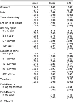
The first and second columns of Table 5 report estimates of the coefficient on gender, schooling, job location, seniority, experience, a time trend, and various time-varying firm vari-ables for the basic and mixed duration models. As is typical with duration analysis, positive coefficients indicate a higher probability of employment termination or, conversely, shorter job duration. Standard errors, reported in parentheses, were computed using the covariance matrix of estimated model pa-rameters given by the inverse of minus the Hessian matrix.
Estimates of the basic (the “Base” column in Table 5), mixed (“Mixed”) and simultaneous (“SIM”) models tell very simi-lar stories about the determinants of employment duration in France. Males keep their job longer, education is associated with a lower probability of job termination, and employment relationships are less stable in the metropolitan area of Paris. For the latter, the magnitude of the coefficients indicates that the probability of losing a job in any year is about 20% higher in Paris.
Table 2. Summary Statistics for Employment Duration (in years)
Mean SD Min Q25 Q50 Q75 Max
2.12 3.12 .08 .25 .83 2.58 19.00
n=989,215
Table 3. Summary Statistics at the Job Level
Men (68%) Women (32%)
Mean SD Mean SD
Censored .15 .36 .13 .34
Lives in Île de France .30 .46 .35 .48
Experience in years
(when spell begins) 12.40 10.40 10.86 9.86
n=989,215
Table 4. Summary Statistics of Annual Data
Men (69%) Women (31%)
Mean SD Mean SD
(log) Wage 4.37 .66 4.11 .69
Capital stock (million FF) 15.70 92.97 10.95 74.16
Number of employees (thousand) 7.88 30.29 5.56 23.93
Total sales (million FF) 7.85 27.59 5.29 21.06
First difference in log-capital stock .09 .51 .10 .50
First difference in log-sales .07 .33 .08 .33
n=2,484,039
Table 5. Estimation Results, Hazard Equation
Base Mixed SIM
Constant 1.249 1.268 1.089
(.017) (.017) (.018)
Male −.069 −.069 −.061
(.003) (.001) (.003)
Years of schooling −.045 −.045 −.045
(.001) (.001) (.001)
Lives in Île de France .192 .191 .210
(.003) (.003) (.003)
Seniority spline
0–2nd year −.763 −.576 −.573
(.002) (.003) (.003)
2–5th year −.093 −.071 −.069
(.002) (.002) (.002)
5–10th year −.059 −.024 −.024
(.002) (.002) (.002)
10th year+ −.054 −.037 −.035
(.003) (.004) (.004)
Experience spline
0–5th year −.105 −.110 −.106
(.001) (.001) (.001)
5–10th year −.061 −.074 −.069
(.001) (.001) (.001)
10–20th year −.016 −.020 −.017
(.001) (.001) (.000)
20–30th year −.021 −.025 −.021
(.001) (.001) (.000)
30th year+ .061 .060 .057
(.001) (.001) (.000)
Time trend .024 .023 .025
(.000) (.001) (.000)
First difference
in log-capital stock −.065 −.064
(.000) (.000)
First difference
in log-sales −.146 −.145
(.003) (.003)
n=989,215
NOTE: Standard errors are in parentheses.
Dostie: Job Turnover and the Returns to Seniority 197
Table 6. Estimation Results, Wage Equation
OLS1 OLS2 Mixed SIM
Constant 2.961 3.125 3.186 2.782
(.002) (.003) (.015) (.016)
Male .229 −.012 −.024 −.031
(.001) (.002) (.003) (.003)
Years of schooling .039 .038 .041 .040
(.000) (.000) (.001) (.001)
Lives in Île de France .216 .216 .142 .140
(.001) (.001) (.001) (.001)
Seniority spline
0–2nd year .042 .042 −.008 −.053
(.001) (.001) (.001) (.001)
2–5th year .020 .020 .008 .005
(.001) (.001) (.000) (.000)
5–10th year −.002 −.002 −.008 −.008
(.000) (.000) (.000) (.000)
10th year+ −.002 −.003 −.008 −.005
(.000) (.000) (.000) (.000)
Male×experience .936 .895 .858
(.010) (.018) (.031)
Experience spline
0–5th year .050 .031 .034 .038
(.002) (.000) (.002) (.002)
5–10th year .035 .022 .019 .019
(.001) (.000) (.001) (.001)
10–20th year .016 .010 .010 .009
(.000) (.000) (.000) (.001)
20–30th year .005 .003 .003 .003
(.000) (.000) (.000) (.001)
30th year+ −.007 −.004 .003 .000
(.000) (.000) (.000) (.000)
Time trend .008 .009 .008 .008
(.000) (.000) (.000) (.000)
First difference
in log-sales −.004 .008 .008
(.001) (.001) (.001)
First difference
in log-capital stock .010 .020 .020
(.001) (.001) (.001)
n=989,215
NOTE: Standard errors are in parentheses.
The impact of seniority and experience is also as expected. Taking into account individual unobserved heterogeneity flat-tens the seniority profile, as can be seen by comparing the co-efficients on the seniority spline in the “Base” and “Mixed” columns in Table 5, but the interpretation remains the same. The first 2 years on a job are associated with an important re-duction in the probability of job termination (−.576 for “0–2nd year” in the “Mixed” column). This indicates that the probabil-ity of job termination is cut in half in each of the first 2 years on a job. This probability keeps falling as seniority increases, but at a much lower rate in the following years. The story is simi-lar with experience. Results show that individuals are sorted in more stable employment relationship as they gain labor mar-ket experience. The effect is again stronger for the first 2 years and gradually dies off after 20 years on the job market. We see the opposite effect after 30 years of experience, due to people getting out of the job market.
Time-varying firm characteristics are found to be important. Increases in both sales and the size of the firm as measured by its capital stock are associated with a lower probability of job termination. Finally, unobserved individual heterogeneity in the job duration equation is found to be significant, although its impact on other coefficients is not dramatic (σθ3 =.546 in the “Mixed” column of Table 7).
Table 7. Variance Components Parameter Estimates
BASE Mixed SIM
Individual heterogeneity variance components,θ,θ
σθ1 .159 .219
(.001) (.002)
σθ2 .989 1.136
(.029) (.045)
σθ3 .546 .563
(.003) (.003)
ρθ1,θ2 −.734 −.747
(.004) (.004)
ρθ1,θ3 −.013
(.011)
ρθ2,θ3 −.345
(.006)
Job heterogeneity variance components,η,η
ση1 .378 .370
(.000) (.005)
ση2 30.345 6.167
(2.583) (.117)
ρη1,η2 .458 .456
(.002) (.002)
λ1 −.020
(.008)
λ2 .013
(.001) Autoregressive error structure
κ1 .202 .180
(.001) (.001)
σu .630 .441 .398
(.000) (.000) (.000)
NOTE: Standard errors are in parentheses.
5.2 Wage Determination
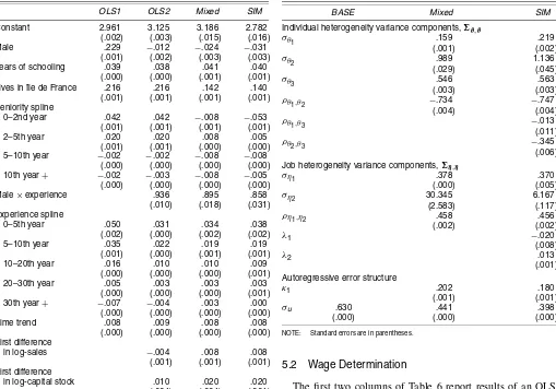
The first two columns of Table 6 report results of an OLS estimation of the wage equation, first in its conventional form and then with additional covariates related to labor demand. We also add a gender interaction to experience, to take into account different life-cycle returns to experience between men and women in the second specification. Typical results are ob-tained for gender, returns to education, and job location for both sets of results. Not surprisingly, men are found to earn more than women, as indicated in the “OLS1” column. However, as shown by the positive interaction term between gender and experience in the other columns, the gap grows wider as indi-viduals gain experience. Looking at the “SIM” column, the in-terpretation is that although returns to experience for women are about 3.8% for their first 5 years on the job market, returns for men are moderately higher at 7.1%(1.858×.038). The returns to an additional year of education are about 4%, and salaries are found to be higher in the Paris metropolitan area. The coef-ficient on the time trend is stable across different specifications and indicates that real wages grew on average by 1% a year between 1978 and 1996. Note that all results for other parame-ters are robust to the inclusion of time dummies instead of a time trend.
Now turning to the returns to specific and general human capital, we find that returns to 10 years of seniority are a lit-tle less than 15% in the OLS regression. The first striking result is obtained by observing how these returns collapse when unob-served heterogeneity is included in the wage equation. Taking into account individual and job unobserved heterogeneity re-duces the returns to seniority to close to zero. When we estimate
the model simultaneously to take into account the endogeneity of seniority, returns to seniority are in fact negative for the first 2 years on a job. This is in stark contrast to returns to experi-ence, which, although diminishing somewhat after taking into account unobserved heterogeneity, still average 4% a year for the first 5 years on the labor market and 2% for the following 5 years in the simultaneous model. It is well known that returns to seniority are pretty low in France (see Abowd et al. 1999), but our estimates are even lower than those reported in previous studies.
Turning to the coefficients on time-varying firm variables, we report in Table 6 that positive changes in sales lower the probability that workers will quit their current job. This is the first time it has been possible to assess the influence of labor demand indicators on employment at the employer–employee match level. As discussed earlier, one interpretation of this re-sult is that these positive changes in sales are indicative of firm labor demand. But one could also argue that these factors are taken into account in the workers’ mobility decisions; positive changes in sales could be used to predict a higher future wage, or a higher probability of promotion within the firm. At this stage one cannot distinguish between these two hypotheses. However, another striking result is that those changes in sales have almost no impact on the wage level.
Finally, in Table 7 we present parameter estimates for the unobserved heterogeneity components. We first note that indi-vidual and job unobserved heterogeneity components are sig-nificant. Significant unobserved job heterogeneity in returns to seniority was also reported by Abowd et al. (1999) and Lillard (1999). The relatively high parameter estimate for ση2 indi-cates that although average returns to seniority are close to zero, actual ranges for those returns are much wider. More in-terestingly, we report in the “SIM” column that both correla-tions between unobserved individual heterogeneity components from the wage equation and those from the hazard equation (ρθ1,θ3 andρθ2,θ3) are significantly different from 0. Both are negative, which suggests that both high-wage and high-wage– growth workers tend to have longer job duration. Also note that bothλ1 andλ2 are statistically significant. This indicates that
good job matches, through either higher starting wage or su-perior wage growth throughout the job, also last longer. Based on these significant correlations, we can reject exogeneity of seniority in the wage equation.
6. CONCLUSION
In this article we estimate simultaneously the wage and job duration processes for a longitudinal sample of French workers from 1978 to 1996 to obtain estimates of the returns to seniority that are not potentially biased by the endogeneity of seniority in the wage equation. We find that taking into account unobserved individual and job heterogeneity considerably lowers the re-turns to seniority estimates. Moreover, these unobservables are significantly correlated across the wage and employment du-ration equations. Taking this correlation into account actually causes the returns to seniority to become negative in the first few years on a job, a result corroborated by a recent study also on French data by Kramarz (2003). Negative returns to seniority for the first few years on a job are consistent with a view of the
job market in which most wage growth comes from switching to higher-paying jobs, especially early in one’s career.
Overall, the foregoing results lend credence to theories that accord greater importance to job search and job matching as determinant of wage level and wage growth, because returns to seniority are found to be very small, even negative. Firm-specific capital does not seem to be important, and human cap-ital would be easily transferable from firm to firm. It remains to be seen what applying our methodology on similar U.S. data would yield. In fact, there is no reason for the returns to senior-ity to be the same in Europe as in the U.S. (Wasmer 2003).
Finally, we find that changes in sales have an important ef-fect in reducing the hazard rate in the mobility equation and a somewhat smaller impact on wages. Therefore, the mobility decision depends on more factors besides demographic charac-teristics and unobserved heterogeneity. We plan on exploring this decision even further in future research by disaggregating our sales data along product lines. It should also be interest-ing to decompose sales shocks into its permanent and tempo-rary components. However, as we noted in our discussion of the results, interpretation of the coefficients on firm-side variables would be helped by the development of theoretical models of the firm linking its employment and wage policies to events on the product market at the micro level. We expect the develop-ment of such models to be spurred by the availability of linked employer–employee datasets.
Another avenue for future research is to decompose the un-observed job-match heterogeneity component into its firm and “pure” job-match components. It would be interesting to get posterior expectations for the firm and individual random ef-fects and aggregate these at the industry level, especially for the job duration equation.
ACKNOWLEDGMENTS
The author acknowledges financial support from the Na-tional Science Foundation (grant SES 99-78093 to Cornell Uni-versity). The author thanks John Abowd, Robert Clark, Gary Fields, Robert Hutchens, George Jakubson, Raji Jayaraman, Joan Moriarty, and three anonymous referees for very helpful comments. All remaining errors are the author’s alone.
[Received May 2002. Revised February 2004.]
REFERENCES
Abowd, J. M., Kramarz, F., and Margolis, D. N. (1999), “High-Wage Workers
and High-Wage Firms,”Econometrica, 67, 251–333.
Abraham, K., and Farber, H. (1987), “Job Duration, Seniority, and Earnings,” American Economic Review, 77, 278–297.
Altonji, J., and Shakotko, R. A. (1987), “Do Wages Rise With Job Seniority?” Review of Economic Studies, 54, 437–459.
Altonji, J., and Williams, N. (1997), “Do Wages Rise With Job Seniority? A Re-assessment,” Working Paper 6010, National Bureau of Economic Research. Anderson, P. M., and Burgess, S. M. (2000), “Empirical Matching Function:
Estimation and Interpretation Using State-Level Data,”Review of Economics
and Statistics, 82, 93–102.
Buchinsky, M., Fougère, D., Kramarz, F., and Tchernis, R. (2003), “Interfirm Mobility, Wages, and the Returns to Seniority and Experience in the U.S.,” mimeo, UCLA.
Hutchens, R. M. (1989), “Seniority, Wages and Productivity: A Turbulent
Decade,”Journal of Economic Perspectives, 2, 49–64.
Dostie: Job Turnover and the Returns to Seniority 199
Jiang, J. (1998), “Consistent Estimators in Generalized Linear Mixed Models,” Journal of the American Statistical Association, 93, 720–729.
Kramarz, F. (2003), “Wages and International Trade,” Discussion Pa-per DP3936, Center for Economic Policy Research.
Lee, Y., and Nelder, J. (1996), “Hierarchical Generalized Linear Models,” Journal of the Royal Statistical Society, Ser. B, 58, 619–678.
Lillard, L. A. (1999), “Job Turnover Heterogeneity and Person-Job-Specific
Time-Series Wages,”Annales d’Économie et de Statistique, 55–56, 183–210.
Meron, M. (1988), “Les Migrations des Salariés de l’État: Plus Loin de Paris,
Plus Près du Soleil,”Économie et Statistique, 214, 3–18.
Searle, S. R., Casella, G., and McCulloch, C. E. (1992),Variance Components,
New York: Wiley.
Topel, R. (1986), “Job Mobility, Search, and Earnings Growth: A
Reinterpre-tation of Human Capital Earnings Functions,” inResearch in Labor
Eco-nomics, Vol. 8, ed. R. Ehrenbrerg, Greenwich, CT: JAI Press, pp. 199–233. (1991), “Specific Capital Mobility and Wages: Wages Rise With Job
Seniority,”Journal of Political Economy, 99, 145–176.
Wasmer, E. (2003), “Interpreting European and U.S. Labour Market Dif-ferences: The Specificity of Human Capital Investments,” Discussion Pa-per DP3780, Center for Economic Policy Research.