Full Terms & Conditions of access and use can be found at
http://www.tandfonline.com/action/journalInformation?journalCode=vjeb20
Download by: [Universitas Maritim Raja Ali Haji] Date: 11 January 2016, At: 22:12
Journal of Education for Business
ISSN: 0883-2323 (Print) 1940-3356 (Online) Journal homepage: http://www.tandfonline.com/loi/vjeb20
A Survey Data Response to the Teaching of Utility
Curves and Risk Aversion
Jeffrey Hobbs & Vivek Sharma
To cite this article: Jeffrey Hobbs & Vivek Sharma (2011) A Survey Data Response to the Teaching of Utility Curves and Risk Aversion, Journal of Education for Business, 86:2, 59-63, DOI: 10.1080/08832321003774780
To link to this article: http://dx.doi.org/10.1080/08832321003774780
Published online: 23 Dec 2010.
Submit your article to this journal
Article views: 41
JOURNAL OF EDUCATION FOR BUSINESS, 86: 59–63, 2011 CopyrightC Taylor & Francis Group, LLC
ISSN: 0883–2323
DOI: 10.1080/08832321003774780
A Survey Data Response to the Teaching of Utility
Curves and Risk Aversion
Jeffrey Hobbs
Appalachian State University, Boone, North Carolina, USA
Vivek Sharma
University of Michigan-Dearborn, Dearborn, Michigan, USA
In many finance and economics courses as well as in practice, the concept of risk aversion is reduced to the standard deviation of returns, whereby risk-averse investors prefer to minimize their portfolios’ standard deviations. In reality, the concept of risk aversion is richer and more interesting than this, and can easily be conveyed through theoretical or applied examples. The authors offer an example of a 2-asset choice problem in which risk-averse investors ought to prefer the asset with not only a higher standard deviation but also a lower expected return. A corresponding survey of 131 respondents confirmed this preference.
Keywords: kurtosis, risk aversion, skewness, standard deviation
INTRODUCTION
The concept of risk aversion underpins all of finance. When teaching finance courses to students, faculty members gen-erally assume that investors have concave utility functions and are thus risk averse, resulting in the risk-return tradeoff, whereby riskier assets are discounted more (i.e., require a higher rate of return as compensation) than less risky assets. Usually, what follows is a reduction of this concept to simple mean–standard deviation space, whereby an asset’s expected return is calculated as the probability-weighted mean of all possible outcomes and its risk is calculated as the standard deviation of those outcomes. Ipso facto, the prescription is for investors to prefer assets that, all else equal, have (a) higher mean returns or (b) lower standard deviations of returns.
This treatment simplifies the issue of risk aversion both mathematically and intuitively, and thus it is commonly used as the basis for teaching and practice (see many finance text-books, including Jordan and Miller [2009]). Moreover, the mean–standard deviation framework extends to other areas of the field. The most notable example of this is portfo-lio theory, where the concepts of the efficient frontier and
Correspondence should be addressed to Vivek Sharma, University of Michigan-Dearborn, Department of Accounting and Finance, 19000 Hub-bard Drive, 9B, FCS, Dearborn, MI 48126, USA. E-mail: vatsmala@ umich.edu
two-fund separation are derived from the use of standard de-viation as the primary measure of an asset’s risk. In practice, the widespread use of the Sharpe Ratio (and its theoreti-cal analogue, the Sharpe Optimal Portfolio) as a measure of investment performance is also consistent with these as-sumptions. However, there is considerable evidence that the unconditional return distributions cannot be adequately char-acterized by mean and variance alone. For example, Merton (1980) showed that if instantaneous returns are normally dis-tributed, then the price process is lognormal and, unless the measurement interval is very small, the simple returns are not normal. This implies that higher moments such as skewness and kurtosis may be important for investment decisions. The seminal work of Kraus and Litzenberger (1976) and Harvey and Siddique (2000) showed how investors’ preference for positive skewness in stock returns may be priced in assets. Mitton and Vorkink (2007) and Boyer, Mitton, and Vorkink (2008) provided empirical evidence suggesting that skew-ness of individual securities may also influence investors’ portfolio decisions. Additionally, Xing, Zhang, and Zhao (2007) found that portfolios formed by sorting on a measure of skewness generate cross-sectional differences in returns. In a similar spirit, Ditmar (2002) investigated whether kur-tosis influences investors’ expected returns. To summarize, investors’ utility from investing in risky assets depends on higher order moments of returns than simply the mean and standard deviation.
60 V. SHARMA AND J. HOBBS
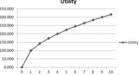
FIGURE 1 Utility curve. The figure illustrates the utility curve for an investor who has a fractional power utility function of the form U(W)= 10000∗√W, which sets the utility of 1 unit of wealth at 100, 4 units at 200,
9 units at 300, and so forth.
In the present paper we offer a simple example of a two-asset choice problem that shows, by contradiction, the short-comings of the mean–standard deviation paradigm. In the example, we assume that the investor exhibits risk aversion (more specifically, a fractional power utility function). The potential payoffs to the two assets are such that one has both a higher expected return and a lower standard deviation than the other. Despite this, the investor gains more in expected utility by buying the low-return, high-risk asset than by se-lecting the high-return, low-risk asset—the exact opposite of what is usually taught in finance. The paper then details the results of a survey asking investors to choose between the two assets in the example. After controlling for age, gender, financial literacy, employment status, and overall wealth, we found that risk aversion is the lone variable that predicts asset choice with statistical significance. Additionally, this choice corresponds to the results of our example, suggesting that investors recognize the importance of skewness and kurtosis in their investment decisions. Last, the paper advises practi-tioners and instructors to carefully weigh the implications of asset choice based strictly on mean and standard deviation, especially in light of the investors’ preference for positive skewness and fatter than normal tails that so often manifest in real-life investments and thus violate the assumption that returns follow a Gaussian probability distribution.
EXAMPLE OF TWO-ASSET CHOICE
Assume that an investor has a fractional power utility function of the form U(W)=10000∗√W, which sets the utility of 1
unit of wealth at 100, 4 units at 200, 9 units at 300, and so forth. Assume further that the investor’s initial wealth (W) is equal to 4 (utility =200). Figure 1 shows the graph of the investor’s utility function, where wealth ranges from 0 to 10. We now assume that the investor is presented with the following two mutually exclusive choices: (a) Investment A provides an equal probability of increasing the investor’s wealth by 0, 1, 2, 3 or 4 units; or (b) Investment B has a 4%
TABLE 1
Return Moments and Utility Gains
Probability
Note.This Table show the return moments and utility gains for an investor presented with the following two mutually exclusive choices: (a) Investment A provides an equal probability of increasing the investor’s wealth by 0, 1, 2, 3, or 4 units; or (b) Investment B has a 4% probability of reducing the investor’s wealth to zero (return of –4), a 66% chance of increasing the investor’s wealth by 2 units, and a 30% chance of increasing the investors wealth by 3 units. For Asset A, E(r)=2.000,SD=1.414, skewness=0.000, kurtosis=–1.300, E(Utility Gain)=43.195. For Asset B, E(r)=2.060, SD=1.318, skewness =–3.782, kurtosis=14.969, E(Utility Gain)= 41.039.
probability of reducing the investor’s wealth to zero (return of –4), a 66% chance of increasing the investor’s wealth by 2 units, and a 30% chance of increasing the investors wealth by 3 units. The return moments and utility gains from these two assets are shown in Table 1. Under this scenario, Investment A’s uniform distribution of returns, ranging from 0 to 4, yields an expected return of 2.000 and a standard deviation equal to the square root of 2 (1.414). Investment B, by contrast, yields an expected return of 2.06 and a standard deviation of 1.318. What is not often discussed are the higher order moments. In our example, the skewness of Asset A is 0.000, in contrast with –3.782 for Asset B. Similarly, the kurtosis measure is –1.300 for Asset A and 14.969 for Asset B. In most discussions of investments, the potential buyer is advised to choose Asset B, owing to its combination of a higher expected return and a lower standard deviation than Asset A. However, our skewness and kurtosis measures indicate that if investors’ conception of risk is primarily associated with extreme negative outcomes, this concern may outweigh the differences in expected return and standard deviation and thus determine Asset A to be the superior choice. In addition, under the set of assumptions outlined, we can also show through simple calculations that Investment A yields the higher expected utility gain (43.195 for Asset A versus 41.0039 for Asset B), despite what at first glance looks like an inferior risk–return structure.
The previous example serves as a relatively simple way to illustrate, through the concept of utility curves and higher order moments, that standard deviation is an imperfect measure of risk. Given that Asset A has a lower expected
RISK AVERSION 61
return than does Asset B, it follows that if standard deviation were a perfect measure of risk, then Asset B’s lower standard deviation would make it the preferable investment. The fact that Asset A is instead the superior choice proves by con-tradiction that standard deviation is an imperfect measure of risk, given the assumptions in our example. We subsequently discuss these assumptions and relate them to real-world in-vestments in more detail.
SURVEY INCORPORATING THE TWO-ASSET EXAMPLE
Though much theoretical and empirical work has been done regarding the nonnormality and skewness of asset return distributions (for examples, see Levy and Duchin, 2004; Mandelbrot, 1963), we attempt to extend this line of research by presenting the aforementioned example to a sample of un-dergraduate and graduate-level students. Doing this allows us to investigate it in more detail; in particular, we cast aside our assumptions about investor wealth and utility curves and fo-cus instead on which of the two assets the respondents prefer. We reproduce the survey below:
1. What is your age? 2. What is your gender?
3. Have you ever enrolled in an introductory finance course?
4. Are you employed more than 20 hours per week? 5. On a scale of 1 to 5, how risk-averse do you consider
yourself to be when it comes to investing money (1=
I very much try to avoid risk, 5=I don’t care about risk)?
6. On a scale of 1 to 5, how financially wealthy do you consider yourself to be (1=Very wealthy, 5 =Not wealthy at all)?
7. Two investments are offered to you. Both require zero money down at the beginning.
If you choose Investment #1, you have an equal chance of these five outcomes: 1) breaking even (no gain or loss), 2) increasing your total wealth by 25%, 3) increasing your total wealth by 50%, 4) increasing your total wealth by 75%, or 5) doubling your total wealth (increase of 100%).
If you choose Investment #2, you have a 4% chance of losing everything you own, a 66% chance of increasing your total wealth by 50%, and a 30% chance of increasing your wealth by 75%. If you had a choice of one or neither—but not
both—of these two investments, which would you choose?
a. I would choose Investment #1 b. I would choose Investment #2 c. I would choose neither
Because the possible payoffs represent such a substan-tial percentage of the respondents’ wealth as to preclude the possibility of rewarding or penalizing them in the same proportions, we asked the students to answer the questions honestly—as if the choice they faced was real. By controlling for age, gender, financial literacy, employment, and wealth (these factors have been examined before with varying re-sults; see Ho, 2009; van Praag and Booij, 2009), we hope to be able to study their effects on asset choice as well as the effect of each respondent’s level of risk aversion.
RESULTS
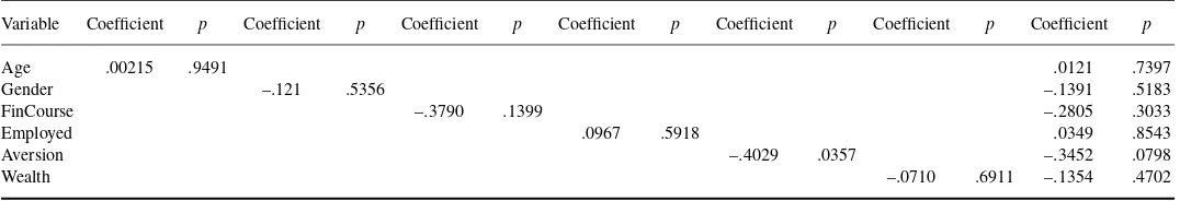
We received responses from 131 students (91 men). The ages of the respondents ranged from 20 to 50 years, but were primarily concentrated in the early and mid twenties. Of the 131 respondents, 78 chose Asset A, 51 chose Asset B, and 2 chose neither asset. Table 2 shows the results of univariate logistic regressions of asset choice on each of the six variables as well as a multiple logistic regression incorporating all six variables. In both cases, Aversion is the only variable that is statistically significant (at the 5% level when asset choice is regressed on aversion alone and at the 10% level when choice is regressed on all six). As we hypothesized, the coefficient on aversion is negative; low scores represent a greater degree of risk aversion and thus a greater likelihood of choosing Asset A, where no loss of wealth is possible. For all regressions, we omitted the two respondents who chose neither Asset A nor B—however, both respondents were relatively risk averse, with one answering “1” and the other answering “2” on the risk-aversion question. The results of the survey reinforce the idea that for people who are more risk-averse—and whose utility functions thus have a greater degree of curvature—standard deviation is an inappropriate measure of risk. For such investors, the importance of the left tail of the distribution outweighs that of the right tail by such an extent that they often choose a lower return, higher standard deviation option as long as the left tail is censored. In our survey, the respondents who put themselves into the highest and second-highest risk aversion categories choose Asset A over Asset B by a margin of 36 to 11.
IMPLICATIONS AND CONCLUSION
Markowitz (1952) and Tobin (1958) established a mean-variance framework of asset valuation based on the assump-tion that asset returns derive from the Gaussian (or a simi-lar, two-parameter and symmetric) probability distribution. While much research has subsequently focused on depar-tures from this assumption (for examples, see Mandelbrot, 1963; Pyle and Turnovsky, 1970), it is an assumption that is nevertheless still very common in teaching and practice.
TABLE 2
Logistic Regressions of Asset Choice
Variable Coefficient p Coefficient p Coefficient p Coefficient p Coefficient p Coefficient p Coefficient p
Age .00215 .9491 .0121 .7397
Gender –.121 .5356 –.1391 .5183
FinCourse –.3790 .1399 –.2805 .3033
Employed .0967 .5918 .0349 .8543
Aversion –.4029 .0357 –.3452 .0798
Wealth –.0710 .6911 –.1354 .4702
Note.Regression coefficients correspond to the probability that the respondent will choose Asset A, which has a lower expected return and higher standard deviation than Asset B but which also has no chance of loss. “Gender” is given a value of 1 if the respondent is a woman and –1 if the respondent is a man, “FinCourse” is given a value of 1 if the answer is “No” and –1 if the answer is “Yes”, and “Employed” is given a value of 1 if the answer is “No” and –1 if the answer is “Yes.” Lower values of “Aversion” correspond to higher levels of risk aversion, and low values of “Wealth” indicate that the respondents consider themselves financially wealthy.
62
RISK AVERSION 63
The purpose of this paper is to show how, using a simple example of two-asset choice, the instructor or practitioner can convey the concept of risk in a way that goes beyond the standard mean-variance framework. The concept can then be extended rather easily to include examples of skewness, kur-tosis or general nonnormality, including the fat-tailed nature of many investments, and the hazards of ignoring them while assessing risk (see the Global Financial Crisis of 2008–2009). Moreover, the results of the survey suggest that although stan-dard deviation is taught as the primary measure of financial risk, most respondents do consider higher moments of return distributions when choosing between investments.
REFERENCES
Boyer, B., Mitton, T., & Vorkink, K. (2008).Expected idiosyncratic skew-ness. Unpublished manuscript.
Dittmar, R. F. (2002). Nonlinear pricing kernels, kurtosis preference, and evidence from the cross section of equity returns.Journal of Finance,57, 369–403.
Harvey, C., & Siddique, A. (2000). Conditional skewness in asset pricing tests.Journal of Finance,55, 1263–1296.
Ho, H. (2009). An experimental study of risk aversion in decision-making under uncertainty.International Advances in Economic Research,15, 369–377.
Jordan, B., & Miller, T. (2009).Fundamentals of investments: Valuation and management. New York, NY: McGraw-Hill.
Kraus, A., & Litzenberger, R. (1976). Skewness preference and the valuation of risk assets.Journal of Finance,31, 1085–1100.
Levy, H., & Duchin, R. (2004). Asset returns’ distributions and the invest-ment horizon.Journal of Portfolio Management,30, 44–62.
Mandelbrot, B. (1963). The variation of certain speculative prices.Journal of Business,36, 394–419.
Markowitz, H. M. (1952). The utility of wealth.Journal of Political Econ-omy,60, 151–156.
Merton, R. (1980). On estimating the expected return on the market: An exploratory investigation.Journal of Financial Economics,8, 1–39. Mitton, T., & Vorkink, K. (2007). Equilibrium underdiversification and the
preference for skewness.Review of Financial Studies,20, 1255–1288. Tobin, J. (1958). Liquidity preference as a behavior toward risk.Review of
Economic Studies,25, 65–86.
Pyle, D., & Turnovsky, S. (1970). Safety-first and expected utility maximiza-tion in mean-standard deviamaximiza-tion portfolio analysis.Review of Economics and Statistics,52, 75–81.
Van Praag, M., & Booij, A. S. (2003).Risk aversion and the subjective time discount rate: A joint approach. CESinfo paper 923.
Xing, Y., Zhang, X., & Zhao, R. (2007). What does individual op-tion volatility smirk tell us about future equity returns? Unpublished manuscript.