AN INTEGRATED INVENTORY MODEL WITH TRANSPORTATION IN
A DIVERGENT SUPPLY CHAN AND UNSTABLE LEAD TIME AND
SETUP COST
Siti Zulfa Choirun Nisak, Nughthoh Arfawi Kurdhi, Sutanto
Department of Mathematics, Sebelas Maret University
ABSTRACT. This research presents single-vendor multi-buyers model with unstable lead ti e a d setup ost a d t a spo tatio i di e ge t supply hai . The e do ’s concern is on crashing of the setup cost, and buyers is on reducing lead time. The vendor manufactures products and delivers them to the buyers located in different locations by a fleet of vehicles with identical capacity. The lead time demand is normally distributed. Excluding transportation time, the lead time component of buyers can be reduced by adding crashing cost. Lead time demand per unit time on buyers are normally distributed. The purpose of this research is to formulate an integrated single-vendor multi-buyers model to determined the optimal solution of order quantity, safety factor, lead time, shipment frequency and routing decision which has been illustrated through a numerical example.
Keyword: integrated inventory model, unstable lead time, unstable setup cost, service level constraint, partial backorder
1.
INTRODUCTION
Inventory management is main component in order a company can run
well.
I e to y a age e t is used to fi d the ight a ou t of p odu t’s ua tity
and the right timing to order products in order to reduce holding cost. At first
inventory management is managed separately by vendor and buyer, but in recent
years many researchers developed integrated inventory management model by
vendor and buyers. Goyal [1] is the first researcher who developed integrated
vendor-buyer inventory model.
In integrated model there will be lead time from buyers order until
products arrived. Ben-Daya and Raouf [2] added crashing cost into model in order
to reduce lead time. Winston [3] explained, it is possible for buyers to order in lead
called backorder when all
uye s illi g to ait p odu t’s a i al. Se o d, alled
lostsales when all buyers refused to wait produ
t’s a i al, a d thi d alled pa tial
backorder when some buyers willing to wait and the rest refused. Ouyang and Wu
[4] added shortage cost into model. Shortage cost is cost which emerged due
to loss of profits and decreasing costumers level credibility then resulting loss
of ostu e s. Sho tage ost is ha d to esti ate e ause it’s
hard to estimate loss
of profits which are effects from product stockout and decreasing costumer level
credibility, so that researchers (Jha and Shanker [5], Ouyang and Wu [4], Wei and
Qiu [6]) replace shortage cost with service level constraint.
Jha and Shanker [5] described integrated inventory single-vendor multi
buyers model with transportation in divergent supply chain under service level
o st ai t. It’s assu
med that all buyers willing to wait. After products had been
finished manufactured then distributed to buyers in several routes with identical
capacity vehicles.
This research developed an integrated inventory with transportation in
divergent supply chain under service level constraint refers to Jha and Shanker [5]
as well as unstable lead time and setup cost refers to Jaggi and Arneja [7] on partial
backorder case refers to Ni
et al
[8]. Furthermore, the optimal order quantity,
safety factors, lead time of buyers and shipment frequency per production cycle,
setup cost of vendor and efficient routes are determined simultaneously by
solving the combined integrated inventory problem and vehicle routing problem
(VRP) using a coordinated two-phase iterative approach.
2.
NOTATION AND ASSUMPTIONS
The following notations and assumptions are used to defined the problem.
Some additional notations and assumptions will be listed later when they are
2.1
Notations
�
number of buyers indexed from
to
�
, index denotes vendor
.
mathematical expectation
+
maximum value of and , i.e.
+= �ax{ , }
For the
−
th buyer
= , , … , �
average demand per unit time
ordering cost per order
�
unit purchase cost
ℎ
holding cost rate per unit time
reorder point
order quantity (decision variable)
safety factor (decision variable)
lead time (decision variable)
transportation time for an order to arrive at buyer from the vendor
(decision variable)
proportion of demand that are not met from stock so
−
is the
service level.
expected demand shortages at the end of buyer’s cycle
lead time demand, which is normally distributed with finite mean
and standard deviation
� √
, where
�
denotes the standard deviation
of demand per unit time,
~�
, � √
For the vendor
production rate,
>
= ∑
�=setup cost per setup (decision variable)
unit production cost (
<
�, ∀
)
ℎ
holding cost rate per unit time
number of lots delivered from the vendor to each buyer (shipment
frequency) in a production cycle, which is same for all buyers, a positive
integer (decision variable)
For vehicle routing
number of routes indexed from to (decision variable)
route
: −
−
− ⋯ − (� ) −
, where
is the
index of the -th buyer visited and
�
≤ � ≤ �
is the number of buyers
in the -th route. Every route starts and finishes at the vendor (decision
variable)
length of route
, = , , … ,
fixed cost of using a vehicle on a route
variable cost per unit distances
vehicle capacity
average speed of vehicle
[image:4.595.150.460.249.710.2]distances between location and
,
∀ , = , , … , �
.
2.2
Assumptions
1.
Buyers orders a lot size
= , , , … , �
and the vendor
manufactures
units with a finite production rate
>
in one
setup but ship in quantity
= ∑
�=over
times using identical
capacity vehicles to meet the demands of all the buyers. The vehicles
on all routes are dispatched simultaneously at the interval of the
uye ’s o
o a e age o de i g y le ti e, i.e.
⁄ = ⁄ =
⋯ =
��
⁄
⇒
=
⁄
.
2.
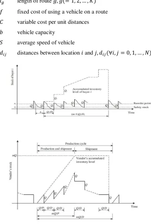
Each buyer reviews inventory using continuous reviews policy and places
an order whenever inventory level falls to the reorder point (Figure 1.).
The reorder point is equal to expected demand during lead time plus
safety stock, that is
=
+ � √
where is safety factor for buyer
.
3.
The setup cost
for the vendor consists of mutually independent
components. The -th component has a normal cost and minimum
cost and a crashing cost when te normal cost reduces to minimum
cost. Arranging such that
≤
≤ ⋯ ≤
, crashing of the setup
cost starts from its first component as it acquires the minimum unit
crashing cost, then the component and so on.
4.
Let
,= ∑
=be the total normal setup cost without crashing and
be the reduced setup cost when component crashed to their minimum
cost, where
= , , , … ,
and given
=
− ∑
=−
, =
, , … ,
and setup crashing cost per cycle
is given as
(
) =
∑
=.
5.
The lead time of buyer has
+
mutual independent components.
The first component s are controllable while the
+
th component
is fixed transportation time from the vendor to buyer . The -th
,
, normal duration
,and a crash cost per unit time
,. Further,
without loss of generality, we assume that
,≤
,≤ ⋯ ≤
,, ∀ .
6.
The controllable lead time component of each buyer are crashed one at a
time starting with the least crashing cost
,, ∀
component and so on.
7.
Let
,= ∑
= ,+ ∑
= ,+ , = , , … ,
and
,be the
length of lead time for buyer with components
, , … ,
crashed to their
minimum
duration,
the
,= ∑
= + ,+ ∑
=+ , = ,
, … , , ∀ .
The lead time crashing cost
per cycle of the th buyer
for a given
∈ [
,,
, −]
is given by
=
,(
, −− ) +
∑
=− ,(
,−
,), ∀ .
8.
If a shortened lead time is requested by a buyer then the extra cost incurred
by the vendor will be fully transferred to that buyer. Therefore, lead time
crashing cost is a cost component of the buyer.
9.
Loading/unloading time is included in the travel time between vendor
–
buyers.
3.
MODEL FORMULATION
This section will explain about model formulation of total expected cost per
unit time for buyers, total expected cost per unit time for vendor, total transportation
cost per unit time and joint total expected cost per unit time.
3.1
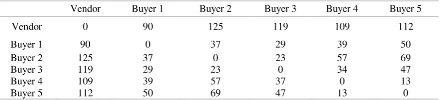
Total expected cost for vendor.
Vendor manufactured the item in quantity of
in one production cycle and delivered and each buyer will receive it in lots each
size
’s such that
=
⁄
for
= , , … , �.
Therefore, the expected length
of production cycle for vendor is
⁄ .
The total expected cost of the vendor
consists of production setup, crashing setup cost and inventory holding cost
−
= � √ �
where
�
= �
− [ − �
]
,
�
and
�
respectively are standard normal
and
CDF
, so the expected number of
backorders per cycle is
� √ �
and expected number of lostsales is
−
� √ �
. Therefore the expected holding cost per year is
ℎ
�[
⁄
+ � √
+
−
� √ �
]
. So, with total buyer ,
=
⁄
, the total expected cost per unit time for the th buyer consists of ordering
cost, holding cost and lead time crashing cost.
�
,
=
�+ ℎ
�[
+
� √ ] +
(3.2)
3.3
Total expected transportation cost per unit time
. The item produced as the
vendor is delivered to the buyers using identical capacity vehicles. The vehicles
combine the deliveries of several buyers into efficient routes and dispatched
simultaneously on all the routes at a common average ordering intervals. The
routing cost of a vehicle consists of a fixed cost which is incurred each time a tour
initiated and a variable cost dependent on the distance traveled. The fixed cost may
include the vehicle rental cost or any other fixed cost which do not depend on the
load size, the route, the number of stops on the route,etc. (Jha and Shanker [5]).
The expected transportation cost per unit time is
=
+ ∑
=.
(3.3)
3.4
Joint total expected cost per unit time.
The joint total expected cost per unit time
for the vendor-buyers integrated system is the sum of total expected cost of the
vendor, total expected cost of the buyer and expected transportation cost so the
problem to be solved is to minimized
, , , … ,
�,
,
, … ,
N, ,
= [
� + ( � )+ ∑ ( +
�=) + (
+ ∑
=)] + ∑ ℎ
�= �[
⁄
+
−
� √ �
] +
ℎ
[
−
− + ]
(3.4)
3.5
Service Level Constraint
Shortage cost is cost which emerged due to loss of profits and decreasing
costumers level credibility then resulting loss of costumers. Shortage cost is
ha d to esti ate e ause it’s
hard to estimate loss of profits which are effects
from product stockout and decreasing costumer level credibility, so that
researchers (Jha and Shanker [5], Ouyang and Wu [4], Wei and Qiu [6]) replace
shortage cost with service level constraint. SLC puts a limit on the proportion
of demands not met from stocks, which should not exceed a specified value.
The SLC for buyer can be obtained as the ratio of expected demand
shortages at the end of cycle and quantity available for satisfying the demand
� √ �
≤
(3.5)
4.
SOLUTION TECHNIQUE
4.1
Solving The Integrated Inventory Problem
To find minimum total expected cost of
( , ,
,
, )
we have to
find optimal solution from variable decision
, , , ,
. Temporarily ignored
service level constrain (SLC) on all buyers from the equation (3.2) and assumed that
vehicle routes are known, which makes the transportation cost component of the total
expected cost as a function of similar to the ordering cost component of the buyers.
For fixed
, ,
and
∈ [
,,
, −], ∀
, the joint total expected cost per unit time
will have minimum value when safety factor of all buyers are zero. Since the function
, ,
, ,
is linear with respect to
, it could be taken as concave as well
as convex too. Therefore,
can be treated as fixed cost item. Now, for fixed
, , ,
) take partial derivatives of
, ,
, ,
with respect to
a�d ∈ [
,,
, −], ∀
respectively, and obtain
� , , ,…, �, , ,…, �,� ,�
= − [
� + ( � )
+ ∑ ( +
�) + (
+
=
∑
=)] + ∑ ℎ
�= �+
ℎ[
−
− + ]
(4.1)
and
� , , ,…, �, , ,…, �,� ,
�
= −
,+ ∑ ℎ
��
− ⁄ �
=
(4.2)
Hence, for fixed
,
,
, , , … ,
�,
,
, … ,
�, � ,
is convex in
since
� , , ,…, �, , ,…, �,� , �=
[
� + ( � )+ ∑ ( +
�) + (
+
=∑
=)] >
However, for fixed
,
,
, , , … ,
�,
,
, … ,
�, � ,
is concave
in
∈ [
,,
, −], ∀
, because
� , , ,…, �, , ,…, �,� ,
�
= −
ℎ
�
�
− ⁄< , ∀
Therefore, for fixed
,
, the minimum joint total expected cost per unit time occurs
at the end points of the interval
∈ [
,,
, −], ∀
.
Therefore,
, , , … ,
�,
,
, … ,
�, � ,
is convex in
for fixed
a�d ∈ [
,,
, −], ∀
. As a result, the necessary condition for
to be optimal
are
∗≤
∗−
dan are
∗≤
∗+
.
On the other hand, by setting (4.1) equal to zero, we obtain
= [
[� +� �
� + ∑�= (� + )+( + ∑��= �)]
�∑�= ℎ � +ℎ [ −�� − +��]
]
/
, ∈ [
,,
, −].
(4.3)
Thus for fixed
∈ [
,,
, −], ∀
,
,
and , if of equation (4.3) satisfies
the SLC from equation (3.5) on all buyers for their zero safety factor, then this and
= , ∀
is optimal and the SLC of all buyers are inactive.
On the other hand for fixed
,
,and
∈ [
,,
, −], ∀
, if
from
equation (4.1) doesn’t satisfy at least one of the buyer’s SLC in equation (3.2) for safety
factors as zero, then is not optimal and SLC on one or more buyer will turn out active.
Therefore for fixed and
∈ [
,,
, −], ∀
to find optimal and safety factor of
all the buyers with active SLC will be using Langrange multiplier technique. The
Langrangian function of the joint total expected cost function is written
= [
� + ( � )+ ∑ ( +
�=) + (
+ ∑
=)
] +
∑ ℎ
�= �[
⁄
+
− � √ �
]
+ ℎ
[
−
− + ] +
∑
∈�� [ � √ �
−
]
(4.4)
where
�
is Langrange multiplier associated with buyer (buyer with active SLC). The
set of buyers with active SLC can be checked by SLC of each buyer one by one for the
safety factor defined as zero and from equation (4.3). Let
∈
and
∈
denote
set of buyers with active SLC and set of buyers with inactive SLC, respectively. If
buyer
, = , , … , �
, follows
� √L
i� �
i/
> ∀
, for
=
then
∈
otherwise
∈
. For fixed and
∈ [
,,
, −], ∀
to obtained optimal solution of
and
for buyers with active SLC with solution to the set equation
�
� = ,
�
�
= ,
�
�� = , ∀
Thus,
��
�
= − [
� + ( � )
+ ∑ ( +
�=) + (
+ ∑
=)
] +
∑ ℎ
�= �+
ℎ[
−
− + ] − ∑
∈��
=
(4.5)
��
�
= ℎ
�� √ − �
√ [ − Φ
] = , ∀
(4.6)
��
��
=
√ �
− �
= , ∀
(4.7)
[
� + ( � )+ ∑ ( +
�=) + (
+ ∑
=)
] + ∑
∈�ℎ �[ −Φ� √ �]−
∑ ℎ
�= �+
ℎ[
−
− + ] =
(4.7)
Thus, by solving equation (4.7) we get
=
∑ ∈ [ −�� ] � � √ +√[∑ ∈ [ −�� ] � � √ ] + [ − − + ]+
∑�= � +}[ � + �
+∑�= (� + )+ + ∑ = ]
[ − − + ]+ ∑�= �
(4.8)
From (4.7), we have
�
=
� √�, ∀
.
(4.9)
The optimal solution of and
can be obtained by taking initial value of
from equation (4.3) then solving equation (4.8) and (4.9) iteratively until convergence,
for fixed and
∈ [
,,
, −], ∀ ,
and
. From procedures described above
optimal value of
∗and
∗can be obtained for fixed routes,
∈ [
,,
, −], ∀
, and
. Based on the convexity and concavity behavior of objective function with respect
to the decision variables the Algorithm 4.1 is developed to find the global optimal
solution for the safety factor, order quantity, and lead time of each buyer, and setup
cost and number of deliveries in one production cycle for known vehicle routes.
Algorithm 4.1
Solving the integrated inventory problem for known vehicle routes.
1.
Set
∗= ∞
and shipment frequency
= .
2.
For each buyer
= , , … �
perform 3
3.
For each
= , , , , … ,
perform 3.1 to 3.4
3.1
Set lead time of buyer to
,∀ = , , … ,
resulting from crashing of
first components and perform step 3.2 to step 3.4 By keeping lead time
fixed at
,∀ = { , , … , �}\{ }
for all other buyers.
3.2
Compute shipment lot size
, ,using equation (4.3).
3.3
If
, ,satisfies the SLC from equation (3.5) of all buyers for safety foctor
, ,
= , ∀ = { , , … , �}
, then set
r
, ,= , ∀
and go to step 3.4
Otherwise follow step 3.3.1 to step 3.3.5 to find shipment lot size
, ,and safety factor
, ,∀
of the buyers with active SLC.
3.3.1
Identify the buyers with active SLC as follows. If the buyer
∈
otherwise
∈
. Take safety factor of buyer with inactive SLC as
zero .
3.3.2
Start with
, ,=
, ,.
3.3.3
Substitute
, ,into equation (4.9) to evaluate
�
, ,,, ∀ ∈
then find
, ,,by checking the standard loss table function table
and hence
Φ
, ,,from the standard normal table.
3.3.4
Utilize
�
, ,,and
Φ(
, ,,), ∀
to determine
, ,from equation
(4.8).
3.3.5
Repeat 3.3.3 and3.3.4 by setting
, ,=
, ,and
, ,,=
,
, ,
, ∀
until no change occurs in the values of
, ,and
, ,∀
.
3.4
Compute
the
corresponding
joint
total
expected
cost
, ,
,
, ,,
, ,,
, ,, … ,
�, ,
,
, ,, …
,, …
�,,
,,
using
equation (3.4).
3.5
Find
�i�
= , ,…
{
, ,
,
, ,,
, ,,
, ,, … ,
�, ,
,
, ,, …
,, …
�,,
,,
}.
Let
(
,
,
, … ,
�,
,
, … ,
� ,, ) =
�i�
= , ,…
{
, ,
,
, ,,
, ,,
, ,, … ,
�, ,
,
, ,, …
,, …
�,,
,,
}
then
∗is the optimal lead time for buyer for fixed .
3.6
Find
�i�
= , ,…
{
, ,
, , , … ,
�
,
,, , …
�,
,,
}.
Let
(
,
,
, … ,
�,
,
, … ,
�, ) =
�i�
= , ,…
{
, ,
, , , … ,
�
,
,, , …
�,
,,
}
then
∗3.7
Take the optimal lead time of all buyers and optimal setup cost for fixed
as
∗, ∀ ,
∗and follow solution procedure described in 3.2 and
3.3
to
find
∗,
∗,
∗, … ,
�∗and
corresponding
(
∗,
∗,
∗, … ,
�∗
,
∗,
∗, … ,
∗�,
∗,
∗)
is the optimal solution for fixed
.
3.8
If
(
∗,
∗,
∗, … ,
�∗
,
∗,
∗, … ,
∗�,
∗,
∗) ≤
∗
,
then
set
∗=
(
∗,
∗,
∗, … ,
�∗
,
∗,
∗, … ,
∗�,
∗,
∗), =
(
∗,
∗,
∗, … ,
�∗,
∗,
∗, … ,
∗�,
∗,
∗) =
(
∗ −,
− ∗,
− ∗, … ,
� − ∗,
− ∗,
− ∗, … ,
� − ∗,
− ∗,
−
∗
)
then
(
∗,
∗,
∗, … ,
�∗
,
∗,
∗, … ,
∗�,
∗,
∗)
is
the optimal solution.
3.10
Determine the optimal order quantity for each buyer using the relationship
∗
=
∗⁄ , ∀
,
then
(
∗,
∗,
∗, … ,
�∗
,
∗,
∗, … ,
∗�,
∗,
∗)
gives
the optimal solution for order quantity, safety factor, lead time of each
buyer, and the number of deliveries in one production cycle to all buyers.
4.2
Solving Vehicle Routing Problem
The optimal value of
is used as input to solve vehicle routing problem (VRP)
using VRP solver which based on Clark-Wright Algorithm. The solver takes input as
distance matrix between each pair of location, order quantity of buyers, and capacity
vehicle. As result, set of routes found, each route will be bidirectional. The vehicle
dispatches from vendor to a set of buyers on a route alongside clockwise (CW) and
counterclockwise (CCW), by comparing transportation time between CW and CCW
routes, route with less transportation time chosen as the route for the next iteration.
4.3
Solving Integrated Inventory Model with Transportation
To solve the integrated inventory problem with transportation cost, the following
algorithm has been proposed to obtain the optimal solution.
Algorithm 4.2
1.
Assume direct shipment between vendor an the buyers. This give as many route
as the number of buyers. (
: − − , = = , , … �
).
2.
Using the routes information find the number of routes, length of each route
and transportation time from the vendor to each buyer. Solve the integrated
inventory problem with help of Algorithm 4.2. This gives the order quantity of
each buyer as one of the outputs.
3.
Take the optimal order quantity of the buyers as input for the VRP solver and
run the VRP solver to obtain set of routes.
4.
Find the cumulative travel distances from vendor to all buyers along each CW
route and CCW route.
5.
For each route, select CW or CCW sequence of route along which cumulative
travel distance from the vendor to all buyers in the sequence has smaller value.
6.
Repeat Step 2
–
Step 5 until the outputs of the integrated inventory problem
5.
NUMERICAL EXAMPLE
The example below taken from Jha and Shanker [5] and Jaggi and Arneja [6].
Here are data for vendor.
= 5
unit per year,
= $ 5
per unit and
ℎ
=0.2.
Data for buyers are written in Table 1, Table 2 is Lead time components, Table 3 is
Setup Cost components and Table 4 is Distance matrix. The vehicle available has the
following characteristics:
= $
per vehicle,
= $ .
per mile,
= 7
units
and
=
miles per day.
-0.022905, 1.026858, 1.0461561, 0.259723
}, order quantity = {237.164, 1185.82,
189.731, 474.329, 237.164}, shipment frequency = 2, setup cost = 2100, and JTEC
= 17003.8
Table 1. Data for buyers
[image:14.595.88.539.405.477.2]Table 2. Data for lead time component
[image:14.595.87.541.526.629.2]Table 3. Data for setup cost component
Table 4. Distance matrix
Buyers (unit per year) � (unit per day) ($ per order) − (%) �($ per unit) ℎ
1,5 1000 7 20 96 25 0.2
2 5000 18 30 97 20 0.2
3 800 10 25 98 22 0.2
4 2000 13 15 99 28 0.2
Lead time component Normal duration
, (days)
Minimum duration ,
(days)
Unit crashing cost
, ($/day)
1 10 4 0.1
2 10 3 1.2
3 8 3 5.0
Setup cost Component
Normal cost
Minimum cost Crashing Setup Cost
1 1300 400 560
2 800 200 1680
3 900 400 3500
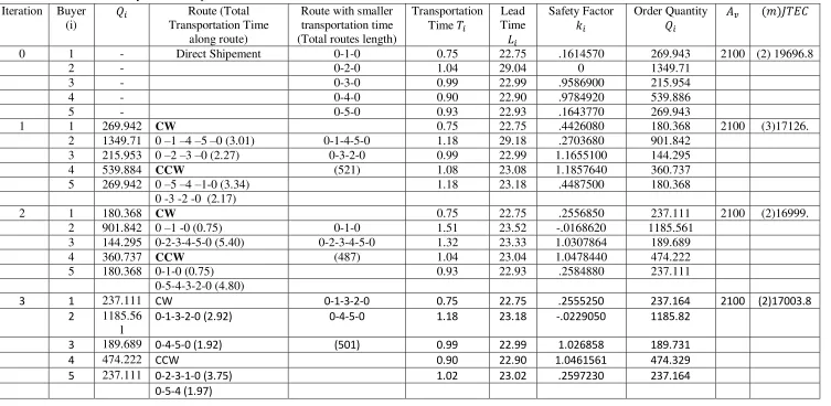
Vendor Buyer 1 Buyer 2 Buyer 3 Buyer 4 Buyer 5
Vendor 0 90 125 119 109 112
Buyer 1 90 0 37 29 39 50
Buyer 2 125 37 0 23 57 69
Buyer 3 119 29 23 0 34 47
Buyer 4 109 39 57 37 0 13
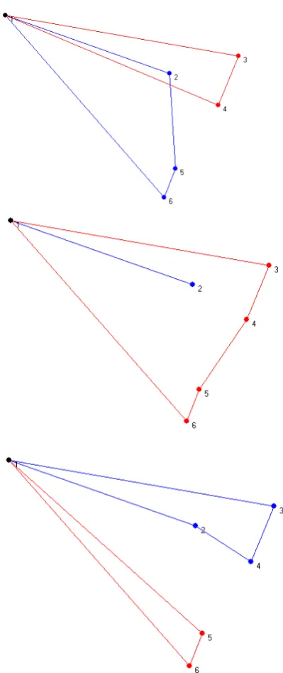
Table 5. Summary of solution procedure Iteration Buyer
(i)
Route (Total Transportation Time
along route)
Route with smaller transportation time (Total routes length)
Transportation Time
Lead Time
Safety Factor Order Quantity
0 1 - Direct Shipement 0-1-0 0.75 22.75 .1614570 269.943 2100 (2) 19696.8
2 - 0-2-0 1.04 29.04 0 1349.71
3 - 0-3-0 0.99 22.99 .9586900 215.954
4 - 0-4-0 0.90 22.90 .9784920 539.886
5 - 0-5-0 0.93 22.93 .1643770 269.943
1 1 269.942 CW 0.75 22.75 .4426080 180.368 2100 (3)17126.
2 1349.71 0 –1 –4 –5 –0 (3.01) 0-1-4-5-0 1.18 29.18 .2703680 901.842 3 215.953 0 –2 –3 –0 (2.27) 0-3-2-0 0.99 22.99 1.1655100 144.295
4 539.884 CCW (521) 1.08 23.08 1.1857640 360.737
5 269.942 0 –5 –4 –1-0 (3.34) 1.18 23.18 .4487500 180.368
0 -3 -2 -0 (2.17)
2 1 180.368 CW 0.75 22.75 .2556850 237.111 2100 (2)16999.
2 901.842 0 –1 -0 (0.75) 0-1-0 1.51 23.52 -.0168620 1185.561
3 144.295 0-2-3-4-5-0 (5.40) 0-2-3-4-5-0 1.32 23.33 1.0307864 189.689
4 360.737 CCW (487) 1.04 23.04 1.0478440 474.222
5 180.368 0-1-0 (0.75) 0.93 22.93 .2584880 237.111
0-5-4-3-2-0 (4.80)
3 1 237.111 CW 0-1-3-2-0 0.75 22.75 .2555250 237.164 2100 (2)17003.8
2 1185.56 1
0-1-3-2-0 (2.92) 0-4-5-0 1.18 23.18 -.0229050 1185.82
3 189.689 0-4-5-0 (1.92) (501) 0.99 22.99 1.026858 189.731
4 474.222 CCW 0.90 22.90 1.0461561 474.329
5 237.111 0-2-3-1-0 (3.75) 1.02 23.02 .2597230 237.164
REFERENCES
[1] Goyal S. K. and Gupta Y.,
Integrated Inventroy Models: the Buyer-Vendor
Coordination
, European Journal of Operation Research 41
,
pp. 261-269, 1989.
[2] Ben-Daya, M. and A. Rouf,
Inventory Model Involving Lead Time as A
Decision Variable
, Journal of Opertional Research Society 45
,
vol. 5, pp.
579-582, 1994.
[3] Winston, W.L.,
Operation Research : Applications and Algorithm
, vol. 3,
California: Wadswort Inc., 2003.
[4] Ouyang, L. Y., N. C. Yeh and K. Wu,
Mixture Inventory Model with
Backorders and Lost Slaes of Variable Lead Time
, Journal of Operational
Research Society
,
vol. 2, pp. 829-832, 1996.
[5] Jha, J. K. and K. Shanker,
An Integrated Inventory Problem with
Transportation in A Divergent Supply Chain Under Service Level Constraint
,
Journal of Manufacturing System 33
,
pp. 462-475, 2014.
[6] Jaggi, C. K. and N. Arneja,
Stochastic Integrated Vendor-Buyer Model with
Unstable Lead Time and Setup Cost
, International Journal of Industrial
Engineering Competitions 2
,
pp. 123-140, 2011.