FORECASTING OF THE ELECTRICITY DEMAND IN LIBYA USING TIME SERIES STOCHASTIC METHOD
FOR LONG-TERM FROM 2011-2022
Thesis
Organized to Meet a Part of the Requirements to Achieve the Master Degree of Mechanical Engineering Department / Specialization of Electrical
Engineering for Renewable Energy
By
SALAH H. E. SALEH S951208518
POST-GRADUATE PROGRAM SEBELAS MARET UNIVERSITY
SURAKARTA 2014
SALAH H. E. SALEH, Student number: S951208507 FORECASTING OF THE ELECTRICITY DEMAND IN LIBYA USING TIME SERIES STOCHASTIC METHOD FOR LONG-TERM FROM 2011-2022. Supervisor I: Prof . Muhammad Nizam, S.T, M.T, Ph.D. Supervisor II: Dr. Miftahul Anwar. Thesis: Mechanical Engineering Deparment, Graduate School, Sebelas Maret University.
Abstract
Forecasting electricity consumption is one of the most important operational issues in order to the facility systems and power sources can be used optimally. Electricity demand forecasting process that will ultimately have an important role in the economic and security of the energy operating system. Looking at the conditions above mentioned, the electrical energy production planning and cost efficiency are needed, in order to provide the maximum benefit for the people and the government. The purposes of this study are: 1) To forecast the electricity for long-term demand from year 2011-2022, based year 2000-2010 datas; 2) To provide mathematical model that can be used as consideration in deciding a particular policy in the field of electricity supply.
The result of analysis shows the determine for long-term demand for generated electricity in Libya in term of data from 2000-2010, used forecasting time series; to provide mathematical data that can be used as consideration in deciding a particular policy in the field of electricity supply. The models found in the SPSS analysis is ARIMA and by Eviews found exponential smoothing model. Forecasting long-term needs 2011-2022, based on data 2000-2010 showed an increase by SPSS, average both Production and Generated reach 5.17 %, and Eviews 5.18 %. The increase Consumption reach average 4.26 % and 5.93 %. Then, an increase average of Population by SPSS 1.41 % and by Eviews 1,35%. The accuracy forecasting about 95% and error degree of freedom about 5%.
Keywords: Forecasting, Electricity, Demand Long-Term From, Time Series, Stochastic Method.
PREFACE
Foremost, I would like to express my gratitude to my supervisors Prof. Muhammad Nizam,. ST., MT., Ph.D for his continuous support during my master study and research, I am extremely grateful for his patience, motivation, and enthusiasm to convey his immense knowledge. He was very helpful for me in the all time of my research and writing of this thesis. Besides to the head of mechanical engineering department Dr.techn Suyitno, ST. MT. I would also like to thank the rest of my thesis Co supervisor Miftahul Anwar S.T., M.T., Ph.D for his encouragement, teaching, and insightful comments. My sincere thanks also go to my classmates in UNS University for their stimulating discussions and helping. And last but not least, I would also like to dedicate this work to my beloved parents and my family for their moral and financial supports, I am totally convinced that I would never come to exist and have succeeded without them. Thank you all. Sincerely.
.
Surakarta, August 2014
CONTENT LIST
Page
TITLE ... i
APPROVAL PAGE ... ii
ABSTRACT ... iv
PREFACE ... v
CONTENT LIST ... vi
TABLE LIST ... vii
FIGURE LIST ... viii
CHAPTER I INTRODUCTION ... 1
1.1Background ... 1
1.2 Problem Statement ... 3
1.3 Research Objectives ... 3
CHAPTER II LITERATURE REVIEW ... 5
2.1 Demand of Electricity ... 5
2.2 Forecasting ... 8
2.3 Types of Forecasting Methods ... 8
2.4 Time Series ... 10
CHAPTER III RESEARCH METHODOLOGY ... 15
3.1 Explanation variable research ... 15
3.2 Research Methodology ... 15
CHAPTER IV DATA ANALYSIS AND DISCUSS ... 18
4.1 Description of The General State of Libya ... 18
4.2 Data Analysis ... 20
4.3 Comparison of Forecasting Results ... 26
CHAPTER V CONCLUSION AND RECOMENDATION ... 41
5.1Conclusion ... 41
5.2Recommendation ... 42
REFERENCE ... 44
APPENDIX ... 46
TABLE LIST
Page
Table 4.1 Growth Population of Libya ... 18
Table 4.2 Description Electricity Usage Data from 2000-2010 ... 19
Table 4.3 Description of electricity production cost from 2000-2010 ... 20
Table 4.4 Description of Power Generated from 2000-2010 ... 21
Table 4.5 Description of Electricity Power Sent to Costumer from 2000-2010 ... 21
Table 4.6 Description of Population from 2000-2010 ... 22
Table 4.7 Model Fit Statistic ... 23
Table 4.8 Result analysis forecasting with ARIMA model parameters ... 25
Table 4.9 Result analysis forecasting with Exponential Smoothing Model parameters by Eviews ... 26
Table 4.10 Model Fit Statistic from 2011-2022 ... 30
Table 4.11 Real and Forecasting of Production Cost ... 31
Table 4.12 Forecasting of electricity demand ... 32
Table 4.13 Growth forecasting of electricity demand ... 32
Table 4.14 Calculation Exponential Smoothing the Production data ... 34
Table 4.15 Calculation Exponential Smoothing the Generated data ... 35
Table 4.16 Calculation Exponential Smoothing the Consumpted data ... 35
Table 4.17 Calculation Exponential Smoothing the Population data ... 36
Table 4.18 Error Calculation Of Moving Average Production ... 37
Table 4.19 Error Calculation Of Moving Average Generated ... 37
Table 4.20 Error Calculation Of Moving Average Consumption ... 38
Table 4.21 Error Calculation Of Moving Average Population ... 38
Table 4.22 Comparison MAD Calculation ... 39
Table 4.23 Error ratio between manual Excel and SPSS ... 40
FIGURE LIST
Figure 2.1 Shows the high-level topology of the electricity transmission network connecting supply (generation) and demand
(customers) ... 6
Figure 2.2 Qualitative Forecasting Methods ... 9
Figure 2.3 Quantitative Forecasting Methods ... 9
Figure 3.1 Flow Chart of Research ... 16
Figure 4.1 Electricity Usage Data from 2000-2010 ... 19
Figure 4.2 Comparison of production costs with SPSS and EViews 7 ... 27
Figure 4.3 Comparison of Generated by SPSS and EViews7 ... 28
Figure 4.4 Comparison Consumption with SPSS and EViews 7 ... 29
Figure 4.5 Comparison of populations with SPSS and EViews 7 ... 29
CHAPTER I INTRODUCTION 1.1 Background
North Africa is the area comprising of Morocco, Algeria, Tunisia, and Libya, with the Sahara desert to the south and the Mediterranean Sea to the north. The climate is dry and warm with annual mean temperatures from 15 °C to 25 °C, with a temperature difference of 20 °C between the coldest and warmest months. Heating is needed during the short winter and there is a large cooling demand during the long summer (Grein et.al, 2007) .
Electricity is an energy which may not be separated from modern society, as in Libya which is always evolving. With an area of almost 1.8 million square kilometers (700,000 sq. mi), Libya is the 17th largest country in the world. Libya has 3900 MTOE (million ton of oil equivalent) oil reserves which is why the Libyan economy depends primarily upon revenues from the oil sector, which accounts for 80% of GDP and 97% of exports. Libya holds the largest proven oil reserves in Africa and also an important contributor to the global supply of light, sweet crude. Apart from petroleum, the other natural resources are natural gas and gypsum. The International Monetary Fund estimated Libya's real GDP growth at 12.2% in 2012 and 16.7% in 2013, after a 60% plunge in 2011 (IMF, 2013).
The World Bank defines Libya as an 'upper middle income economy', along with only seven other African countries. Substantial revenues from the energy sector, coupled with a small population, gives Libya one of the highest per capita GDPs in Africa. This allowed the Libya to provide an extensive level of social security, particularly in the fields of housing and education
A condition which can‟t be evoided because of improved living standards in Libya is the increasing use of electrical energy. Oil is the most important source of energy to supply the power generator. According to (GECL; 2012) the libyan‟s TPES data (Total Primary Energy Supply) in 2004, oil gas have supplied 72.7 % and 26.5% of energy respectively. Fossil fuel accounted for 99.2 % in
Libya. This growing energy consumption is a result of the urbanization process in the region, economic growth, population growth, and industrialization.
What to be done, an increase in demand as the economic growth reflected in, change in life style and increased energy consumption for e.g. Space heating and cooling. The government of libya will face 2050 more pressure on the future energy supply, especially in the residential sector with its increasing cooling and heating demand. In the future, by those reason, the Governments will be forced to more efficient energy use to overcome the increasing energy cost. The installed capacity of power generation has increased. The residential sector is one of the main consumers of electricity. In 2004, 32.3 % of the electricity in Libya was consumed by the residential sector and the power consumption of the industry was 2 %. The power demand from 2003 till 2050 will grow rapidly. The demand of the residential sector is expected to grow by 80 % due to rapid population growth.
Based on the statement mentioned above, allocating precision fuel used for power generation is necessary in order to the consumer electricity needs can be met optimally and efficiently. The amount of power demand during a period of time cannot be calculated certainty, as the result, it will raise the question of how to operate a power system plant continuously which can meet the power demand in any time. If the power delivered from the plant is much larger than the load power demand, then there will be wastage of electricity generation cost at the power company. However if the generated and delivered power are lower or even do not meet the needs of consumers, There will be a local blackout and absolutely its harm to the consumers.
Large-scale electric power cannot be stored but must be raised in accordance with load demand or consumer. Therefore forecasting electricity consumption is one of the most important operational issues in order to the facility systems and power sources can be used optimally. With a good electricity demand forecasting, the quantity and quality of electric power generated can fulfill the needs of consumers.
in the economic and security of the energy operating system. As we know, generating of electrical energy requires a very large cost. Production efficiency and the selection of priorities is necessary to achieve the balanced goals. Moreover, to generate electrical energy is also influenced by political considerations, availability of fuel and qualified human resources in the field of electricity. To achieve a balanced demand, it is important to make a mapping electrical needs for providers in this case is the Libyan government.
Sustainable supply of electric power is a prerequisite to foster all sorts of development in a country. Development of electricity infrastructure is undoubtedly a capital intensive project that needs a careful planning especially when taken future expansion into consideration (Amlabu et al. 2013). Knowing the condition and all the rising electrical problems, the author is interested in researching and analyzing the need for electricity in Libya. Author focuses on electricity demand forecasting and the effort of efficiency so it reduces the supply electricity cost in Libya. In accordance with the framework that has been the author describe above, the author takes the title “Forecasting Of The Electricity Demand In Libya Using Time Series Stochastic Method For Long-Term From 2011-2022”.
1.2 Problem Statement
In this case the limitation issue is crucial in order to the main problem and the object under study can be achieved and the problems remain focus or not widespread. In this study, the writer put focus on:
1) How to determine the long-term demand for electricity in Libya in term of data from year 2011-2022?
2) How to provide mathematical data that can be used as consideration in deciding a particular policy in the field of electricity supply?
1.3 Research Objectives
A reasearch need a goal as a found a mental reference to the problem under study, so that a researcher will work more focus and organize in the conduct of research. The purposes of this study are:
1) To forecast the electricity for long-term demand from year 2011-2022, based year 2000-2010 datas.
2) To provide mathematical model that can be used as consideration in deciding a particular policy in the field of electricity supply.
CHAPTER II LITERATURE REVIEW
2.1Demand of electricity 2.1.1 Demand
Demand means the quantity of a given article which would be taken at a given price. Supply means the quantity of that article which could be had at that price. Defines that demand is the amount of a particular economic good or service that a consumer or group of consumers will want to purchase at a given price. The demand curve is usually downward sloping, since consumers will want to buy more as price decreases. Demand for a good or service is determined by many different factors other than price, such as the price of substitute goods and complementary goods. In extreme cases, demand may be completely unrelated to price, or nearly infinite at a given price. Along with supply, demand is one of the two key determinants of the market price (Aemo, 2012).
2.1.2 Electricity
According to electricity is the set of physical phenomena associated with the presence and flow of electric charge. Electricity gives a wide variety of well-known effects, such as lightning, static electricity, electromagnetic induction and electrical current. In addition, electricity permits the creation and reception of electromagnetic radiation such as radio waves. While based on. electricity is a form of energy resulting from the existence of charged particles (such as electrons or protons), either statically as an accumulation of charge or dynamically as a current.
Based on both describtion of demand and electricity, we could take a conclution to give the meaning that electricity demand is the amount of electricity being consumed at any given time (Aemo, 2012).
metering supply to the network rather than consumption. The benefit of measuring demand this way is that it includes electricity used by customers, energy lost transporting the electricity (network losses), and the energy used to generate the electricity (auxiliary loads).
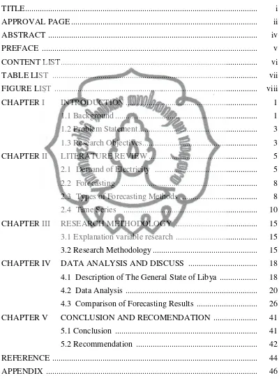
Figure 2.1- shows the high-level topology of the electricity transmission network connecting supply (generation) and demand (customers) (Aemo, 2012)
It also shows the different points at which supply and demand are measured as well as the relative contribution of different types of generation. The electricity (energy) supplied by a generator can be measured in two ways: (Aemo, 2012)
a) Supply „as-generated‟ is measured at the generator terminals, and represents the entire output from a generator.
b) Supply „sent-out‟ is measured at the generator connection point, and represents only the electricity supplied to the market, excluding a generator‟s auxiliary loads.
c) The basis for projecting energy and maximum demand
d) Energy is presented on a sent-out basis. This means that the energy projections include the customer load (supplied from the network) and network losses, but not auxiliary loads.
e) Maximum demand is presented on an as-generated basis. This means that the maximum demand projections (the highest level of instantaneous demand for electricity during summer and winter each year, averaged over a 30-minute period) include the customer load (supplied from the network), the network losses, and the auxiliary loads.
2.1.3 Power distribution system
Generally the types of consumers according to the wearer can be grouped in to the following categories: (Aemo, 2012)
a) Household (domestic/resident), consisting of lighting load, fans, household appliances such as heaters, refrigerators, electric stoves, and others.
b) Business, consisting of lighting loads and other electrical equipment used in commercial buildings or trades such as shops, restaurants, and others.
c) Public / public, consisting of government buildings, street lighting, and social interest users.
d) Industry, consisting of small industrial/household and large industries. The factors that determine the load characteristics are as follows: a) Needs factor
The needs factor is a comparison between the maximum demands with a total load attached or connected to the system. Needs Factor depends on the type and consumer‟s activities, the location and the system of power.
b) Load factor
Load factor is the planned average load ratio on a period of time to the peak load occurring in that period. Load factor only measures variations and does not represent the exact designation of the load duration curve.
2.2Forecasting
A prediction scenario of future events and situations are called forecasts, and the act of making such predictions is called forecasting. Forecasting is the basic facet of decision making in different areas of life. The purpose of forecasting is to minimize the risk in decision making and reduce unanticipated cost.
One of the most important works of an electric power utility is to correctly predict load requirements, In broad terms, power system load forecasting can be categorized into long-term and short-term functions. Long-term load forecasting usually covers from one to ten years based on monthly, yearly values. Explicitly, it is intended for applications in capacity expansion, and long term capital investment return studies.
In simplicity, forecasting is a system for quantitatively determining future load demand. (Amlabu et al. 2013)
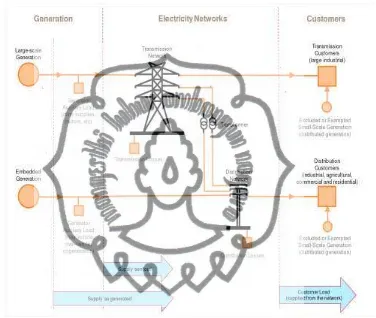
2.3Types of forecasting methods
Qualitative methods: These types of forecasting methods are based on judgments, opinions, intuition, emotions, or personal experiences and are subjective in nature. They do not rely on any rigorous mathematical computations.
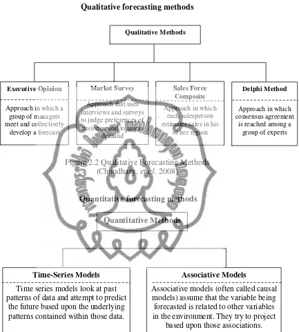
Quantitative methods: These types of forecasting methods are based on mathematical (quantitative) models, and are objective in nature. They rely heavily on mathematical computations. (Choudhary, et al. 2008)
Qualitative forecasting methods
Figure 2.2 Qualitative Forecasting Methods (Choudhary, et al. 2008)
Quantitative forecasting methods
Figure 2.3 Quantitative Forecasting Methods (Choudhary, et al. 2008) Time series models look at past patterns of data and attempt to predict
the future based upon the underlying patterns contained within those data.
Associative Models
Associative models (often called causal models) assume that the variable being forecasted is related to other variables in the environment. They try to project
based upon those associations. Quantitative Methods
2.4Time Series 2.4.1. Definition
A time scries is a collection of observations made sequentially through time Examples occur in a variety of fields, ranging from economics to engineering, and methods of analysing time series constitute an important area of statistics (Chatfileld, 2009).
2.4.2. Objectives of Time Series
There are several possible objectives in analysing a time series these objectives mav be Classified as description, explanation, prediction and control, and will be considered in turn (Chatfileld, 2009). Based Fan (2005), the objectives of time series analysis are diverse, depending on the background of applications. Statisticians usually view a time series as a realization from a stochastic process. A fundamental task is to unveil the probability law that governs the observed lime series. With such a probability law. We can understand the underlying dynamics, forecast future events, and control future, events via intervention. Those arc the three main objectives of time scries analysis.
2.4.3. Components of a Time Series
According (Adhikari, and Agrawal, 2009). A time series in general is supposed to be affected by four main components, which can be separated from the observed data. These components are: Trend, Cyclical, Seasonal and Irregular components. A brief description of these four components is given here.
The general tendency of a time series to increase, decrease or stagnate over a long period of time is termed as Secular Trend or simply Trend. Thus, it can be said that trend is a long term movement in a time series. For example, series relating to population growth, number of houses in a city etc. show upward trend, whereas downward trend can be observed in series relating to mortality rates, epidemics, etc 2.4.4. Time Series and Stochastic Process
attempt to understand the nature of the series and is often useful for future forecasting and simulation.
In time series forecasting, past observations are collected and analyzed to develop a suitable mathematical model which captures the underlying data generating process for the series. The future events are then predicted using the model. This approach is particularly useful when there is not much knowledge about the statistical pattern followed by the successive observations or when there is a lack of a satisfactory explanatory model. Time series forecasting has important applications in various fields. Often valuable strategic decisions and precautionary measures are taken based on the forecast results. Thus making a good forecast, i.e. fitting an adequate model to a time series is vary important. Over the past several decades many efforts have been made by researchers for the development and improvement of suitable time series forecasting models.
A time series is non-deterministic in nature, i.e. we cannot predict with certainty what will occur in future. Generally a time series {x (t), t=0,1,2,..} is assumed to follow certain probability model which describes the joint distribution of the random variable xt. The mathematical expression describing the probability structure of a time
series is termed as a stochastic process. Thus the sequence of observations of the series is actually a sample realization of the stochastic process that produced it.
A usual assumption is that the time series variables xt are independent and
identically distributed (i.i.d) following the normal distribution. However as mentioned in, an interesting point is that time series are in fact not exactly i.i.d; they follow more or less some regular pattern in long term. For example if the temperature today of a particular city is extremely high, then it can be reasonably presumed that tomorrow‟s temperature will also likely to be high. This is the reason why time series forecasting using a proper technique, yields result close to the actual value.
2.4.5. Time Series Models
often intertwined to generate new models. For example, the autoregressive moving average model (ARMA) combines the (AR) model and the (MA) model.
Another example of this is the autoregressive integrated moving average (ARIMA) model, which combine all three of the models previously mentioned. The most commonly used model for time series data is the autoregressive process. The autoregressive process is a difference equation determined by random variables. The distribution of such random variables is the key component in modeling time series.
Data collection techniques for discrete time series can be done in two ways, as described as follows:
1. Through sampling of continuous time series. it means the continuous data is sampled in the same time interval.
2. Through the accumulation of a variable in a period of time. For example, rainfall is usually accumulated over a certain period of time (days, months, etc.).
Mathematical models for stochastic and deterministic dynamic problem:
1. If the value of a future (future value) of a time series can be appropriately determined by a mathematical function, eg: Zt = cos (2πft), it can be called deterministic time series.
2. If the future value can only be described in a probability distribution. It can be called as a stochastic time series.
The basic model used in the time series analysis is ARIMA that can be expressed by a linear combination of observation variables data and independent random variables distributed normally. Based the describe above, the approaches time series that uses to forecasting electricity demand in Libya are:
1. Autoregressive integrated moving average (ARIMA)
considered in this paper is Autoregressive Integrated Moving Average (ARIMA) time series.
2. Exponential smoothing;
Exponential smoothing is probably the widely used class of procedures for smoothing discrete time series in order to forecast the immediate future. This popularity can be attributed to its simplicity, its computational efficiency, the ease of adjusting its responsiveness to changes in the process being forecast, and its reasonable accuracy.
The idea of exponential smoothing is to smooth the original series the way the moving average does and to use the smoothed series in forecasting future values of the variable of interest. In exponential smoothing, however, it is need to allow the more recent values of the series to have greater influence on the forecast of future values than the more distant observations. Exponential smoothing is a simple and pragmatic approach to forecasting, whereby the forecast is constructed from an exponentially weighted average of past observations. The largest weight is given to the present observation, less weight to the immediately preceding observation, even less weight to the observation before that, and so on (exponential decay of influence of past data (Amlabu et al; 2013) .
There are a variety of these methods, such as single exponential smoothing, Holt‟s linear method, and Holt-Winters‟ method and their variations. Although still used in several areas of business and eco-nomic forecasting, these are now supplemented by the other four methods mentioned previously. (Ostertagová, K. et al. 2011) .
2.4.6. To Make sure Stochasic Time Series Analysis
Forecasting accuracy can be measured from the following values: 1. Mean Squared Error (MSE), an average prediction error sum of squares .
2. Mean Absolute Deviation (MAD), is the average absolute value of forecast error .
MAD =
n
r
t Y Yt n 1
1
(2.3)
Note :
Yt = value of observation Yt ' = value estimates
In the method of time series there are a few things to note, first of all is Stationer data, and second is the autocorrelation function and the last is partial autocorrelation function. Stationary time series is a condition where the generation process in determining a time series based on the inconstant mean value and constant variance. In a data, it's possible to be non stationary data because of a constant mean, so to eliminate non-stationary data, the data can be made closer to be stationary by using the differencing distinction method. it can be stabilized by using transformations.
CHAPTER III
RESEARCH METHODOLOGY
3. 1 Explanation of the research variables
The research variables are electricity demand factors. The electricity demand factors are production cost, generated power, consumption and population variables. The relevant research with this research, his done by Saravanan (2012) with the title “India‟s Electricity Demand Forecast Using Regression Analysis and Artificial Neural Networks Based On Principal Components”. The aim of this study deals with electricity consumption in India, to forecast future projection of demand for a period of 19 years from 2012-2030. The eleven input variables used amount of CO2 emission, Population, Per capita GDP, Per capita gross national income, Industry, Consumer price index, Imports, Exports and Per capita power consumption and production cost. (Saravanan, 2012). Based on these studies, this study uses the variable production costs, power generated, consumption and population.
3.2 Research methology
In this research method describes the steps that will be done, as showed in figure 3.1.
Figure 3.1 Flow Chart of Research
The following steps were used in the following analysis: 1. Input Data and Stationary Analysis
2. To test the feasibility of the Model Parameter Estimation
Conducting parameter estimation based on the model obtained through SPSS and EViews software, and testing the significance of parameters to get a significant parameter model.
3. Subsequently forecasting 2011- 2022 years.
CHAPTER IV
DATA ANALYSIS AND DISCUSSION
4.1 Description of the general state of Libya 4.1.1 Population growth Libya
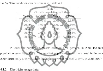
The population in Libya has fluctuated from year to year ranged between 1-2 %. This condition can be seen as in Table 4.1.
Table 4.1
Growth population of Libya Years Value Years Value
2001 1.91% 2006 2.15% 2002 1.93% 2007 2.19% 2003 1.96% 2008 2.10% 2004 2.02% 2009 1.84% 2005 2.07% 2010 1.48%
In 2000 the population growth reached 1.91 percent. In 2001 the total population grew by 1.93 %. The smallest population growth occurred in the year 2009-2010, only 1.48 %. While the highest growth reached 2.19 % in 2006-2007.
4.1.2 Electricity usage data
Based on the survey results revealed statistical data about electricity usage country of Libya. Descriptive statistics were used to explanations include the average, median, mode, standard deviation, minimum and maximum, and number. Electricity usage data used in this study generated, electricity consumption by the public.
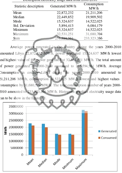
Table 4.2
Description electricity usage data from 2000-2010 Statistic description Generated MW/h Consumption
MW/h
Mean 22,872,232 21,211,206
Median 22,449,852 19,909,502
Mode 15,324,637 14,522,025
Std. Deviation 5,894,413 6,084,179
Minimum 15,324,637 14,522,025
Maximum 32,531,251 31,680,704
Sum 251,594,561 233,323,266
Average power generated in the country during the years 2000-2010 amounted Libya 22,872,232 MW/h, power generated 15,324,637 MW/h lowest and highest value of the power generated at 32,531,251 MW/h. The total amount of power generated in 2000-2010 amounted to 251,594,561 MW/h. Average Consumption in country Libya during the years 2000-2010 amounted to 21,211,206 MW/h, consumption 14,522,025 MW/h lowest and highest values consumption by 31,680,704 MW/h. The total consumption number of years 2000-2010 amounted to 233,323,266 MW/h. Histogram graphics electricity usage data can to be show in the figure 4.1.
Figure 4.1 Electricity Usage Data from 2000-2010 Source: analysis data by SPSS 15 version 2014
Based on the above picture was highest average on the data generated in the last follow consumption data and power usage. In the above data do not indicate a significant change of image variations. The small value of the consumption electricity better than average, median, mode, standard deviation, minimum and maximum shows that the Libyan government has been managing the use of electricity as well as possible.
4.2 Data analysis
4.2.1 Description of data
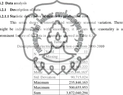
4.2.1.1Statistic descriptive of electricity production cost
This series shows a smooth trend with little seasonal variation. There might be individual series with seasonality, it appears that seasonality is a prominent feature of the data in general as showed in Table 4.3.
Table 4.3
Description of electricity production cost from 2000-2010
N Valid 11
Missing 0
Mean 352,003,663
Median 345,503,222
Mode 235,846,163a
Std. Deviation 90,715,024 Minimum 235,846,163 Maximum 500,655,953
Sum 3,872,040,294
Based on table of 4.3, the mean of production costs from 2000-2010 median of calculating the mean USD 352,003,663, USD 345,503,222, about production costs. Average cost of production in Libya State nearly USD 352,003,663, which means that the cost of electricity used to produce high enough. In the above data indicated that the maximum cost unheard of and lows of USD 500,655,953, USD 235,846,163. Price for 1 MW of electricity production amounted to USD 15.39. Resulting in the production of electricity generated from the average cost of USD 352,003,663.07 is 22,872,232 MW/h.
4.2.1.2Statistic descriptive of power generated
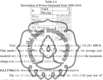
Based on research data known power supply. The data collected from the 2000-2010. The results are detailed in Table 4.4.
Table 4.4
Description of Power Generated from 2000-2010
N Valid 11 incurred only for USD 352,003,663.07 to average the cost is below the maximum charge ever issued for Libyan State 2000-2010.
4.2.1.3Statistic descriptive of electricity power consumption
The use of electric power by the people of the 2000-2010 year low of 14,522,025 MW/h and 31,680,704 MW/h for general centipede average electricity use of 21,211,206.00 MW/h following data table electricity use by the public.
Table 4.5
Description of Electricity Power Sent to Costumer from 2000-2010
Average consumption in the country during the years 2000-2010 amounted Libya 21,211,206 MW/h, consumption 14,522,025 MW/h lowest and highest value of the consumption at 31,680,704 MW/h. The total amount of consumption in 2000-2010 amounted to 233,323,266 MW/h.
4.2.1.4Statistic descriptive of population
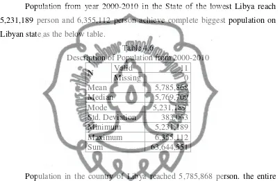
Population from year 2000-2010 in the State of the lowest Libya reach 5,231,189 person and 6,355,112 person achieve complete biggest population on Libyan state as the below table.
Table 4.6
Description of Population from 2000-2010
N Valid 11
Missing 0
Mean 5,785,868
Median 5,769,709 Mode 5,231,189a Std. Deviation 383,063 Minimum 5,231,189 Maximum 6,355,112
Sum 63,644,551
Population in the country of Libya reached 5,785,868 person. the entire population of the year 2000-2010 reached number 63,644,551 person
4.2.2 Goodness-of-Fit Measures
Table of summary statistics for stationary R-square, R-square, root mean square error, mean absolute percentage error, mean absolute error, maximum absolute percentage error, maximum absolute error, and normalized Bayesian Information Criterion. The Normalized Bayesian Information Criterion, as a general measure of the overall fit of a model that attempts to account for model complexity. It is a score based upon the mean square error and includes a penalty for the number of parameters in the model and the length of the series. The penalty removes the advantage of models with more parameters, making the statistic easy to compare across different models for the same series (Norušis,
Table 4.7 Model Fit Statistic Model Stationary
R-squared R-squared RMSE MAPE Production-Model_1 .580 .991 884,1431.741 1.763 Generated-Model_2 .580 .991 57,4491.991 1.763
Consumption-Model_3
-1.757E-16 .958 1,217,524.605 3.815 Population-Model_4 0.000 1.000 4,947.405 .071
Continue Table 4.7
Model MAE MaxAPE MaxAE Normalized
BIC Production-Model_1 6,021,407.853 4.308 19,004,280.541 32.426 Generated-Model_2 391,254.571 4.308 1,234,846.040 26.958
Consumption-Model_3
783,931.280 10.868 3,015,625.100 28.255 Population-Model_4 4,272.438 .125 7,839.250 17.273
Stationary R - squared. A measure that compares the stationary part of the model to a simple average. Variables that have a negative value that is consumption, which means that the model under consideration is worse than the base line model. While the variable production costs, generated, population have a positive value means that the model under consideration is better than the basic model.
R - Squared. Estimates of the proportion of the total variation in the series described by the model. This step is very useful when the series is stationary. All variables have a positive value means that the model under consideration is better than the basic model.
RMSE. Root Mean Square Error. The square root of the mean square error. A measure of how much the series varies depending on the level of its prediction models, expressed in the same units as the dependent series. RMSE of all the variables with the highest consumption variable 1,217,524.605 value and a low of population variable with a value of 4,947.405
As for who has the highest MAPE lowest in the population variable with a value of 0.071
MAE. Mean absolute error. Measures how much the series varies from its level prediction models. MAE is the highest on the production variable value and the lowest 6,021,407.853 population variable with a value of 4,272.438
MaxAPE. Maximum Absolute Percentage Error. The largest estimated error, expressed as a percentage. MaxAPE highest in the variable value consumption by 10.868 and the population with the lowest value of 0.125.
MaxAE. Maximum Absolute Error. The largest estimated error. MaxAE highest in variable production abaout 19,004,280.541 and the lowest values occurring in the population variable with a value of 7,839,250.
Normalized BIC. Normalized Bayesian Information Criterion. General measure overall model fit that tries to explain the complexity of the model. Normalized BIC variables that have high production is a variable with a value of 32,426 and the lowest values occur in the population variable with a value of 17. 273.
4.2.3 Result Analysis ARIMA Model Parameters by SPSS
Result analysis on the variable production cost, power generated, consumption, population, only four variables included in the ARIMA model type. The results of forecasting the variables that could use the model as follows ARIMA.
Table 4.8Result analysis forecasting with ARIMA model parameters
2011 405,504,753 26,348,587 12,993,675 6,103,221 2012 533,397,023 34,658,676 20,602,217 6,154,623 2013 543,774,561 35,332,980 6,237,393 Forecasting
2011 537,150,947 34,902,596 33,396,572 6,448,248.21 2012 571,653,578 37,144,482 35,112,440 6,542,064.89 2013 606,156,210 39,386,368 36,828,308 6,636,576.65 2014 640,658,842 41,628,255 38,544,176 6,731,790.58 2015 675,161,473 43,870,141 40,260,043 6,827,713.79 2016 709,664,105 46,112,028 41,975,911 6,924,353.35 2017 744,166,737 48,353,914 43,691,779 7,021,716.36 2018 778,669,368 50,595,800 45,407,647 7,119,809.92 2019 813,172,000 52,837,687 47,123,515 7,218,641.11 2020 847,674,632 55,079,573 48,839,383 7,318,217.03 2021 882,177,264 57,321,460 50,555,251 7,418,544.77 2022 916,679,895 59,563,346 52,271,119 7,519,631.42
There was gap on data 2011-2012 with the result forecasting on 2011-2012. That happened because of war tragedy in Libya. As long 7 month, in libya have internal conflict, so use electricity consumption can not be forecast as exactly.
Table 4.9. Result analysis forecasting with Exponential Smoothing Model parameters by EViews
Years Production Cost Generated MW/h
Consumption
MW/h Population 2011 405,504,753 26,348,587 12,993,675 6,103,221 2012 533,397,023 34,658,676 20,602,217 6,154,623 2013 543,774,561 35,332,980 6,237,393
Forecasting
2011 537,336,336 34,914,642 34,728,817 6,447,557 2012 571,873,032 37,158,742 37,312,458 6,540,002 2013 606,409,729 39,402,841 39,896,099 6,632,447 2014 640,946,425 41,646,941 42,479,741 6,724,892 2015 675,483,121 43,891,041 45,063,382 6,817,337 2016 710,019,818 46,135,141 47,647,023 6,909,782 2017 744,556,514 48,379,241 50,230,665 7,002,227 2018 779,093,210 50,623,340 52,814,306 7,094,672 2019 813,629,907 52,867,440 55,397,948 7,187,117 2020 848,166,603 55,111,540 57,981,589 7,279,562 2021 882,703,299 57,355,640 60,565,230 7,372,007 2022 917,239,995 59,599,740 63,148,872 7,464,452 Source: Analysis data by EViews
There was gap on empirical data and forecasting. That happened because of war tragedy in Libya. As long 7 month, at libya have internal conflict, so use electricity consumption can not be forecast as exactly.
4.3 Comparison of forecasting results
Comparisons of forecast results are used to obserences the differences of the variables used in this study. This comparison uses two types of analysis software the first is ARIMA Model by SPSS and second is Exponential Smoohting by EViews 7.
4.3.1 Production cost
The comparison of production costs is based on the results of forecasting using SPSS and EViews 7 as in the figure 4.2.
Figure 4.2 Comparison of production costs with SPSS and EViews 7
Based on the Figure 4.2 above shows that forecasting using EViews 7 software has higher expectations than on forecasting using SPSS. This is seen from year to year has predictions starting in the overall of 2011-2022 forecasting results demonstrated the results using EViews higher than in 2022 as SPSS forecasting using EViews 7 which reached USD 917,239,995 greater than using the SPSS reached USD 916,679,895.
4.3.2 Generated
A comparison of forecasting results that were generated using SPSS and EViews 7asin the Figure 4.3.
Years
Figure 4.3 Comparison of Generated by SPSS and EViews7
Based on the Figure 4.3 above shows that forecasting using EViews7 software has higher expectations than on forecasting using SPSS. This is seen from year to year has predictions starting in the 2011-2022 overall forecasting results put the results by using EViews 7 higher than the SPSS as 2022 59,2599,740 MW/h forecasting using EViews 7 achieve greater than using the SPSS reached 59,599,740 MW/h
4.3.3 Consumption
Comparison of forecasting results consumption by using SPSS and EViews 7 as in the Figure 4.4.
P
ower G
en
era
ted
Years
Figure 4.4 Comparison consumption with SPSS and EViews 7
Based on the Figure 4.4 above which shows that forecasting using EViews 7 software has higher expectations than on forecasting using SPSS. This is seen from year to year has predictions starting in the 2011-2022 overall forecasting results put the results by using EViews higher than the SPSS as in 2022 reached 63,148,872 MW/h forecasting using EViews 7 greater than using the SPSS reached 52,271,119 MW/h.
4.3.4 Population
Comparison of population based on the results of forecasting using SPSS and EViews 7 as in the Figure 4.5.
Figure 4.5 Comparison of populations with SPSS and EViews 7
Co
n
su
m
p
ti
o
n
t
Years
p
o
p
u
lat
ion
years
Based on the Figure 4.5 above which shows that forecasting using SPSS software has higher expectations than on forecasting using EViews 7. This is seen from year to year has predictions starting in the 2011-2022 overall forecasting results put the results using SPSS higher than in 2022 EViews 7 like forecasting using SPSS reached 7,519,631 person greater than using EViews 7 which reached 7,464,452 Person.
The difference in the forecasting results using SPSS and EViews are caused by differences in forecasting models. The ARIMA forecasting using SPSS data according forecasting results as the Table 4.10.
Table 4.10 Model Fit Statistic from 2011-2022 by SPSS Years Real of
Consumption MWh Years
Forecasting of demand MWh
2000 14,522,025 2011 33,396,572 2001 15,208,543 2012 35,112,440 2002 15,445,816 2013 36,828,308 2003 16,702,230 2014 38,544,176 2004 17,931,957 2015 40,260,043 2005 19,909,502 2016 41,975,911 2006 21,730,193 2017 43,691,779 2007 23,016,749 2018 45,407,647 2008 27,748,242 2019 47,123,515 2009 29,427,305 2020 48,839,383 2010 31,680,704 2021 50,555,251 2011 12,993,675 2022 52,271,119 2012 20,602,217
Source: analysis data by SPSS 15 version 2014
electricity needs in Libya should not be less than consumption. If that happens, it will shake up the Libyan economy. Besides that, attention should be paid to that the electric power will be lost, as long as we have not resolved the bias in producing electricity, should pay attention to power consumption and loss of electricity, or in other words to meet the demands for electricity in producing electricity it needs to accumulate between electricity consumption and electricity loss.
4.3.6 Production cost in the process of distributing electricity to Libya Production costs for producing electricity to be distributed to consumers as in the Table 4.11.
Table 4.11 Real and Forecasting of production Cost by SPSS Years Real of Production
cost MWh Years
Forecasting of Production cost MWh 2000 235,846,163.4 2011 537,150,947 2001 246,466,479.2 2012 571,653,578 2002 269,796,995.9 2013 606,156,210 2003 291,526,567.8 2014 640,658,842 2004 310,905,609.7 2015 675,161,473 2005 345,503,222.3 2016 709,664,105 2006 369,243,682.4 2017 744,166,737 2007 392,661,722 2018 778,669,368 2008 441,171,910 2019 813,172,000 2009 468,261,988.2 2020 847,674,632 2010 500,655,952.9 2021 882,177,264 2022 916,679,895
4.3.7 Forecasting of electricity demand to determine the long-term from 2011-2022
Forecasting electricity to meet the demand in Libya from year 2011-2022 as Table 4.12 and 4.13.
Table 4.12 Forecasting of electricity demand Years Generated
MWh
Consumption MWh 2011 34,902,596 33,396,572 2012 37,144,482 35,112,440 2013 39,386,368 36,828,308 2014 41,628,255 38,544,176 2015 43,870,141 40,260,043 2016 46,112,028 41,975,911 2017 48,353,914 43,691,779 2018 50,595,800 45,407,647 2019 52,837,687 47,123,515 2020 55,079,573 48,839,383 2021 57,321,460 50,555,251 2022 59,563,346 52,271,119 Source: analysis data by SPSS 15 version 2014
Table 4.13 Growth forecasting of electricity demand Years Generated
Source: analysis data by SPSS 15 version 2014
4.3.8 The Mathematical Model is Based On Forecasting
y = difference between forecasting year target and the initial year Example: - mathematical forecasting of POP for 2017
y = 2017-2000 = 17
The increase in the amount of fuel consumption 2000-2010
Ratio of population = 2010-2000
= 6,355,112-5,231,189
Error if compare with result of forecasting of SPSS
4.3.9 Calculation Exponential Smoothing
The important insight is to know the best method to forecast the electricity demand. Hence, the discussion about error should be added in to the thesis.
Calculate exponential smoothing the first column is time or period and the second column is actual data and third, about forecasted data. To find forecasted data, the first row is average actual data, beginning from 2000 -2010. Still in the third column, the second row calculate forecasting, use this formulation:
(4.2)
Ft = Forecasting value period t
Ft-1 = Forecasting value period t-1
At-1 = actual value forecasting value period t-1 α = smoothing constant
Table 4.14 Calculation Exponential Smoothing the Production data Production
2000 1 235,846,163 352,003,663 -116,157,500 116,157,500 116,157,500.00 116,157,500.00 2001 2 246,466,479 247,461,913 -995,434 995,434 117,152,934.00 58,576,467.00 2002 3 269,796,996 246,566,022 23,230,974 23,230,974 140,383,907.60 46,794,635.87 2003 4 291,526,568 267,473,899 24,052,669 24,052,669 164,436,576.96 41,109,144.24 2004 5 310,905,610 289,121,301 21,784,309 21,784,309 186,220,885.90 37,244,177.18 2005 6 345,503,222 308,727,179 36,776,043 36,776,043 222,996,928.79 37,166,154.80 2006 7S 369,243,682 341,825,618 27,418,064 27,418,064 250,414,993.08 35,773,570.44 2007 8 392,661,722 366,501,876 26,159,846 26,159,846 276,574,839.51 34,571,854.94 2008 9 441,171,910 390,045,737 51,126,173 51,126,173 327,701,012.15 36,411,223.57 2009 10 468,261,988 436,059,293 32,202,695 32,202,695 359,903,707.42 35,990,370.74 2010 11 500,655,953 465,041,718 35,614,235 35,614,235 395,517,941.94 35,956,176.54
2011 497,094,530
Mean 352,003,663
Table 4.15 Calculation Exponential Smoothing the Generated data 2000 1 15,324,637 22,872,233 -7,547,596 7,547,595.82 7,547,595.82 7,547,595.82 2001 2 16,014,716 16,079,397 -64,681 64,680.58 7,612,276.40 3,806,138.20 2002 3 17,530,669 16,021,184 1,509,485 1,509,484.94 9,121,761.34 3,040,587.11 2003 4 18,942,597 17,379,721 1,562,876 1,562,876.49 10,684,637.84 2,671,159.46 2004 5 20,201,794 18,786,309 1,415,485 1,415,484.65 12,100,122.49 2,420,024.50 2005 6 22,449,852 20,060,246 2,389,606 2,389,606.46 14,489,728.95 2,414,954.83 2006 7 23,992,442 22,210,891 1,781,551 1,781,550.65 16,271,279.60 2,324,468.51 2007 8 25,514,082 23,814,287 1,699,795 1,699,795.06 17,971,074.66 2,246,384.33 2008 9 28,666,141 25,344,102 3,322,039 3,322,038.51 21,293,113.17 2,365,901.46 2009 10 30,426,380 28,333,937 2,092,443 2,092,442.85 23,385,556.02 2,338,555.60 2010 11 32,531,251 30,217,136 2,314,115 2,314,115.29 25,699,671.30 2,336,333.75
2011 32,299,839
Mean 22872232.82
Table 4.16 Calculation Exponential Smoothing the Consumpted data Consumption
period N Consumption actual data
6,689,181 6,689,181.00 6,689,181.00 6,689,181.00 2001 2 15208543 15,190,943 17,600 17,599.90 6,706,780.90 3,353,390.45 2002 3 15445816 15,206,783 239,033 239,032.99 6,945,813.89 2,315,271.30 2003 4 16702230 15,421,913 1,280,317 1,280,317.30 8,226,131.19 2,056,532.80 2004 5 17931957 16,574,198 1,357,759 1,357,758.73 9,583,889.92 1,916,777.98 2005 6 19909502 17,796,181 2,113,321 2,113,320.87 11,697,210.79 1,949,535.13 2006 7 21730193 19,698,170 2,032,023 2,032,023.09 13,729,233.88 1,961,319.13 2007 8 23016749 21,526,991 1,489,758 1,489,758.31 15,218,992.19 1,902,374.02 2008 9 27748242 22,867,773 4,880,469 4,880,468.83 20,099,461.02 2,233,273.45 2009 10 29427305 27,260,195 2,167,110 2,167,109.88 22,266,570.90 2,226,657.09 2010 11 31680704 29,210,594 2,470,110 2,470,109.99 24,736,680.89 2,248,789.17
31,433,693 Mean 21211206
Table 4.17 Calculation Exponential Smoothing the Population data 2000 1 5,231,189.00 5,785,868 -554,679 554,679.27 554,679.27 277,339.64 2001 2 5,331,311.00 5,286,657 44,654 599,333.35 599,333.35 199,777.78 2002 3 5,434,293.00 5,326,846 107,447 706,780.75 706,780.75 176,695.19 2003 4 5,541,062.00 5,423,548 117,514 824,294.49 824,294.49 164,858.90 2004 5 5,652,797.00 5,529,311 123,486 947,780.87 947,780.87 157,963.48 2005 6 5,769,709.00 5,640,448 129,261 1,077,041.50 1,077,041.50 153,863.07 2006 7 5,893,738.00 5,756,783 136,955 1,213,996.57 1,213,996.57 151,749.57 2007 8 6,023,053.00 5,880,042 143,011 1,357,007.08 1,357,007.08 150,778.56 2008 9 6,149,620.00 6,008,752 140,868 1,497,875.13 1,497,875.13 149,787.51 2009 10 6,262,667.00 6,135,533 127,134 1,625,008.93 1,625,008.93 147,728.08 2010 11 6,355,112.00 6,249,954 105,158 1,730,167.31 1,730,167.31 157,287.94
6,344,596 Mean 5785868.273
4.3.10 Calculation of Exponential Smoothing
1. First step, input actual data, calculate average actual data then we will get the average
2. Put average as forecast the first time
3. The second time until the next time with calculate by ES formulation
= Ft = Ft-1+ α (At-1 - Ft-1)
Ft = Forecasting value period t
Ft-1= Forecasting value period t-1
At-1= Actual value forecasting value period t-1
α = smoothing constant
4. Until here, calculate about forecasting, and the next step, analysis to make sure forecasting used Mean Absolute Deviation (MAD) so, the calculate the error (actual data – forecasting data) change the error by absolute data, the absolute error is move symbol front of numbers, cumulative is calculation absolute error
5. The mad calculate is number cumulative in the last number divided count of all period
4.3.11 Error Calculation Of Moving Average
Table 4.18 Error Calculation Of Moving Average Production
Years Actual
Production Data Forecast MA=4
Absolute
2004 310,905,610.00 260,909,051.50 49,996,558.50
2005 345,503,222.00 279,673,913.25 65,829,308.75 270,908,363.20 74,594,858.80 2006 369,243,682.00 304,433,099.00 64,810,583.00 292,839,775.00 76,403,907.00 2007 392,661,722.00 329,294,770.50 63,366,951.50 317,395,215.60 75,266,506.40 2008 441,171,910.00 354,578,559.00 86,593,351.00 341,968,160.80 99,203,749.20 2009 468,261,988.00 387,145,134.00 81,116,854.00 371,897,229.20 96,364,758.80 2010 500,655,953.00 417,834,825.50 82,821,127.50 403,368,504.80 97,287,448.20
2011 450,687,893.25 434,399,051.00
MAD 45,068,789.33 43,439,905.10
Table 4.19 Error Calculation Of Moving Average Generated Years Generated
Actual Data Forecast MA=4
Absolute
2004 20,201,794.00 16,953,154.75 3,248,639.25
2005 22,449,852.00 18,172,444.00 4,277,408.00 17,602,882.60 4,846,969.40 2006 23,992,442.00 19,781,228.00 4,211,214.00 19,027,925.60 4,964,516.40 2007 25,514,082.00 21,396,671.25 4,117,410.75 20,623,470.80 4,890,611.20 2008 28,666,141.00 23,039,542.50 5,626,598.50 22,220,153.40 6,445,987.60 2009 30,426,380.00 25,155,629.25 5,270,750.75 24,164,862.20 6,261,517.80 2010 32,531,251.00 27,149,761.25 5,381,489.75 26,209,779.40 6,321,471.60
2011 29,284,463.50 28,226,059.20
MAD 2,928,446.35 2,822,605.92
Table 4.20 Error Calculation Of Moving Average Consumption Years Consumption
Actual Data Forecast MA=4
Absolute
2004 17,931,957.00 15,469,653.50 2,462,303.50
2005 19,909,502.00 16,322,136.50 3,587,365.50 15,962,114.20 3,947,387.80 2006 21,730,193.00 17,497,376.25 4,232,816.75 17,039,609.60 4,690,583.40 2007 23,016,749.00 19,068,470.50 3,948,278.50 18,343,939.60 4,672,809.40 2008 27,748,242.00 20,647,100.25 7,101,141.75 19,858,126.20 7,890,115.80 2009 29,427,305.00 23,101,171.50 6,326,133.50 22,067,328.60 7,359,976.40 2010 31,680,704.00 25,480,622.25 6,200,081.75 24,366,398.20 7,314,305.80
2011 27,968,250.00 26,720,638.60
MAD 2,796,825 2,672,064
Table 4.21 Error Calculation Of Moving Average Population Years Population
Actual Data Forecast MA=4
Absolute
2004 5,652,797.00 5,384,463.75 268,333.25
2005 5,769,709.00 5,489,865.75 279,843.25 5,438,130.40 331,578.60 2006 5,893,738.00 5,599,465.25 294,272.75 5,545,834.40 347,903.60 2007 6,023,053.00 5,714,326.50 308,726.50 5,658,319.80 364,733.20 2008 6,149,620.00 5,834,824.25 314,795.75 5,776,071.80 373,548.20 2009 6,262,667.00 5,959,030.00 303,637.00 5,897,783.40 364,883.60 2010 6,355,112.00 6,082,269.50 272,842.50 6,019,757.40 335,354.60
2011 6,197,613.00 6,136,838.00
MAD 619,761 613,684
The describ in detail to calculate the error of forecasting in 2022. Next, the calculate error forecasting uses Moving Average and make sure uses MAD.
4.3.12 Calculation of ARIMA
The first column is time or period. The second column is t (period or time). The third column are actual data.
1. The first step input actual data
MA =
3. Until here, calculate about forecasting was finish, and the next step, analysis to make sure forecasting used Mean Absolute Deviation (MAD)
4. so, the Calculate the error (actual data – forecasting data)
5. Change the error by absolute data, the absolute error is move symbol front of numbers
6. Cumulative is calculation absolute error
7. The mad calculate is number cumulative in the last number divided count of all period
The last step is calculated the mad and low value it is will be better model to forecasting. Finally the best model.
Table 4.22 Comparison MAD Calculation MAD ARIMA Production 45,068,789 43,439,905 35,956,177 Exponential Smoothing
Generated 2,928,446 2,822,606 2,336,334 Exponential Smoothing Consumption 2,796,825 2,672,064 2,248,789 Exponential Smoothing Population 619,761 613,684 157,288 Exponential Smoothing
Calculate the error to make a sure of result if compare with result of forecasting of SPSS or EViews untill 2022 year by year from 2011-2022 by this formultion:
100
Example: error ratio between manual Excel and SPSS
Table 4.23 Error ratio between manual Excel and SPSS Years Production $ Generated Consumption Population
2011 1,89% 1,89% 0,02% 0,31%
2012 3,25% 3,25% 0,02% 0,59%
2013 4,48% 4,48% 0,02% 0,85%
2014 5,61% 5,61% 0,02% 1,09%
2015 6,64% 6,64% 0,02% 1,31%
2016 7,59% 7,59% 0,02% 1,51%
2017 8,46% 8,46% 0,02% 1,70%
2018 9,27% 9,27% 0,03% 1,87%
2019 10,03% 10,03% 0,03% 2,03% 2020 10,73% 10,73% 0,03% 2,17% 2021 11,38% 11,38% 0,03% 2,30% 2022 11,99% 11,99% 0,03% 2,41%
CHAPTER V
CONCLUSION AND RECOMENDATION
5.1 Conclusion
Based on the research and the result of analysis about forecasting of the electricity demands in Libya using time series Stochastic method for long-term from 2011-2022, we can conclude the following:
We were able to determine the long-term demands for electricity in Libya in term of data from 2000-2010, by using forecasting time series. Time series forecasting method is formulated with time series data. Technical time series: there are two time series, they are deterministic and stochastic time series. Time series deterministic is a forecasting method with time series data where the data must meet the data stationary. This is due to a deterministic time series forecasting are methods appropriately. Terms of stationary data are used as the basis for forecasting the proper method deterministic time series. Studying energy demands at a disaggregated sectoral level for policy purposes. An application to the demand for electricity in Libya shows that alternative policy options for market reforms can be based on reliable long-term forecasts from in-sample parameter estimates of long-run relationships that are useful for decision-making
To provide mathematical data that can be used as consideration in deciding a particular policy in the field of electricity supply, mathematical data that can be used in A stochastic time series is forecasting method assuming there is still a possibility of committing a mistake. The data used for the analysis of stochastic time series does not require stationary requirements.
The research analysis process is a stochastic time series analysis because the data used does not meet the requirements of stationary. On the results of stochastic time series analysis using SPSS, the process runs smoothly. Models found in the SPSS analysis is ARIMA. The results of the analysis of SPSS can be presented.
As for the mathematical models that can be used as a material consideration in deciding a particular policy in the field of power supply,
according to the variables used to adjust and present clearly, that all models have a slight positive direction. Forecasting long-term needs 2011-2022, based on data 2000-2010 showed an increase. That means they need the government in each year to increase production. If not there will be a power shortage that will put a large load on the Libyan economy.
5.2 Recommendation 1) Government
The government should use its power sources carefully. Government also needs to fix the electricity network infrastructure so that electricity needs can be met in Libya for the benefit of society. Because the government of Libya will face 2050 more pressure on the future energy supply, especially in the residential sector with its increasing cooling and heating demands. In the future, according to those reasons, the government will be forced to allow more efficient energy use to overcome the increasing energy cost, make strategies towards a more efficient allocation of resources while taking account of the budgetary “go to the use of renewable energy”.
An application to the demand for electricity in Libya shows that alternative policy options can be based on reliable long-term forecasts of long-run relationships that are useful for decision-making.
Specifically, the forecasts under different scenarios for subsidy removal that reflect the pace of reform can help the government in devising appropriate strategies towards a more efficient allocation of resources. The adoption of a certain scenario to remove problems in electricity market depend on the development of a social protection system most of all efficient functioning of a social safety net requires that the target consumer groups be determined on well-defined criteria.
This will help in designing programs that aim at improving both resource allocation and income distribution.
2) Community
To Libya community, should use adequate electric power alone. Screening for heating or air can be used only if needed, and reduce unnecessary power usage. People when using energy efficiently, they will help the government improve national energy securely. Energy saving is also beneficial to reduce the cost of electricity bills. Particularly in every household, reducing the cost of electricity bills every month can help reduce monthly expenses.
3) The Research
Should be able to explore new ideas and research findings in order to develop a forecasting electricity demand and be able to provide feedback to the use of electricity effective.
REFERENCES
Adhikari, Ratnadip and Agrawal, R. K. 2009 An Introductory Study on Time
serie modeling and forecasting
http://arxiv.org/ftp/arxiv/papers/1302/1302. 6613.pdf
Aemo, 2012, Chapter 2 - Definitions, Process And Methodology, http://www.aemo.com.au/en/Electricity/Forecasting. Viewed June 2012. Amlabu, C.A., Agber, J.U., Onah, C.O., and Mohammed, S.Y. , 2013. Electric
Load Forecasting: A Case Study of the Nigerian Power Sector.
International Journal of Engineering and Innovative Technology (IJEIT). Volume 2, Issue 10
Anoname. General Electricity Company of Libya (GECL), 2012. http://www.gecol.ly/aspx/Statistics.aspx
Anoname. International Monetary Fund. IMF Country Report No. 13/151. Libya: Selected Issues. 2013
Chatfileld, Chris, 2009. The Analysis of Time Series: an Introduction. Sixth Edition, CRC Press LLC 2000 NW. Corporate Blvd, Boca Raton. Florida Choudhary, M.A., Khan, N., Ali, A., and Abbas, A., 2008, Achievability of
Pakistan's 2030 Electricity Generation Goals Established under Medium Term Development Framework (Mtdf): Validation Using Time Series Models and Error Decomposition Technique, Energy 2030 Conference, 2008. ENERGY 2008. IEEE.
Grein, M., Nordell, B., and Al Mathnani, A., 2007, Energy Consumption and Future Potential of Renewable Energy in North Africa, Gas, Vol. 64 (26.5), pp. 0.4
Jianqing, Fan., and Qiwei Yao, 2005. Non Linier Time Series, nonparametric and parametric Method. Springer Science & Business Media, Inc., 233 Spring St., New York, NY 10013, USA
Matei, Demetrescu, 2012., 9. Time series and stochastic processes. University of Bonn
Norušis, Marija J. 2007. The SPSS Guide to Data Analysis. Universitas Michigan
Ostertagová, E., and Ostertag, O., 2011, The Simple Exponential Smoothing Model, The 4th International Conference on Modelling of Mechanical and Mechatronic Systems, Technical University of Košice, Slovak Republic,
Rahman, S., and Hazim, O., 1996. Load Forecasting for Multiple Sites: Development of an Expert System-Based Technique. Electric Power Systems Research, 39:161–169
Saleh, I.M. 2006. Prospects of renewable energy in Libya. international Symposium on Solar Physics and Solar Eclipses (SPSE). Al-Fateh University. Tripoli.
Saravanan, 2012. India‟s Electricity Demand Forecast Using Regression Analysis and Artificial Neural Networks Based On Principal Components. Ictact Journal On Soft Computing, July 2012, Volume: 02, Issue: 04
Soni, A., and Sharma, A. 2013. Electricity Load Forecast for Power System Planning. International Refereed Journal of Engineering and Science (IRJES). Volume 2, Issue 9 (September 2013), PP. 52-57
Vahviläinen, I., Pyykkönen, T. 2005. Stochastic factor model for electricity spot price – the case of the Nordic market, Energy Economics, forthcoming Wakhid, A. Jauhari. 2011. Manajemen Permintaan (Section 2). Teknik Industri
UNS: Surakarta
APPENDIX
Original Data Years Production $ Generated
MW/h
Consumption
MW/h POP
2000 235,846,163 15,324,637 14,522,025 5,231,189 2001 246,466,479 16,014,716 15,208,543 5,331,311 2002 269,796,996 17,530,669 15,445,816 5,434,293 2003 291,526,568 18,942,597 16,702,230 5,541,062 2004 310,905,610 20,201,794 17,931,957 5,652,797 2005 345,503,222 22,449,852 19,909,502 5,769,709 2006 369,243,682 23,992,442 21,730,193 5,893,738 2007 392,661,722 25,514,082 23,016,749 6,023,053 2008 441,171,910 28,666,141 27,748,242 6,149,620 2009 468,261,988 30,426,380 29,427,305 6,262,667 2010 500,655,953 32,531,251 31,680,704 6,355,112 Source: General Electricity Company of Libya
Forecasting by SPSS Years Production $ Generated
MW/h
Consumption
MW/h POP
2011 537,150,947 34,902,596 33,396,572 6,448,248 2012 571,653,578 37,144,482 35,112,440 6,542,065 2013 606,156,210 39,386,368 36,828,308 6,636,577 2014 640,658,842 41,628,255 38,544,176 6,731,791 2015 675,161,473 43,870,141 40,260,044 6,827,714 2016 709,664,105 46,112,028 41,975,911 6,924,353 2017 744,166,737 48,353,914 43,691,779 7,021,716 2018 778,669,368 50,595,800 45,407,647 7,119,810 2019 813,172,000 52,837,687 47,123,515 7,218,641 2020 847,674,632 55,079,573 48,839,383 7,318,217 2021 882,177,264 57,321,460 50,555,251 7,418,545 2022 916,679,895 59,563,346 52,271,119 7,519,631