CLUSTERING OF MULTISPECTRAL AIRBORNE LASER SCANNING DATA USING
GAUSSIAN DECOMPOSITION
S. Morsy*, A. Shaker, A. El-Rabbany
Department of Civil Engineering, Ryerson University, 350 Victoria St, Toronto, ON M5B 2K3, Canada - (salem.morsy, ahmed.shaker, rabbany)@ryerson.ca
Commission III, WG III/5
KEY WORDS: Multispectral, LiDAR, Gaussian, Ground filtering, Histogram, NDVI
ABSTRACT:
With the evolution of the LiDAR technology, multispectral airborne laser scanning systems are currently available. The first operational multispectral airborne LiDAR sensor, the Optech Titan, acquires LiDAR point clouds at three different wavelengths (1.550, 1.064, 0.532 m), allowing the acquisition of different spectral information of land surface. Consequently, the recent studies are devoted to use the radiometric information (i.e., intensity) of the LiDAR data along with the geometric information (e.g., height) for classification purposes. In this study, a data clustering method, based on Gaussian decomposition, is presented. First, a ground filtering mechanism is applied to separate non-ground from ground points. Then, three normalized difference vegetation indices (NDVIs) are computed for both non-ground and ground points, followed by histograms construction from each NDVI. The Gaussian function model is used to decompose the histograms into a number of Gaussian components. The maximum likelihood estimate of the Gaussian components is then optimized using Expectation – Maximization algorithm. The intersection points of the adjacent Gaussian components are subsequently used as threshold values, whereas different classes can be clustered. This method is used to classify the terrain of an urban area in Oshawa, Ontario, Canada, into four main classes, namely roofs, trees, asphalt and grass. It is shown that the proposed method has achieved an overall accuracy up to 95.1% using different NDVIs.
* Corresponding author
1. INTRODUCTION
Over the past two decades, airborne LiDAR data have been used in urban applications (Yan et al., 2015). Numerous studies have focused on extracting one object type in urban scenes, such as separation of ground from non-ground points in order to generate digital terrain models (DEMs) (Bartels et al. 2006), building extraction (Huang et al., 2013), road extraction (Samadzadegan et al., 2009) and curbstones mapping (Zhou and Vosselman, 2012). The number of extracted classes has been extended to three main urban classes, including ground, vegetation and buildings (Samadzadegan et al., 2010). Nowadays, multi-classes extraction is a very important topic for building 3D city models, maps updating and emergency purposes. However, most of recent studies focus on geometric characteristics of the LiDAR data (Xu et al., 2014; Blomley et al., 2016).
Recently, Teledyne Optech has launched the world’s first airborne multispectral LiDAR sensor “Optech Titan”. This sensor acquires LiDAR data in three channels C1, C2, and C3 at wavelengths of 1.550 m, 1.064 m, and 0.532 m, respectively. The data are acquired at pulse repetition frequencies (PRF) ranges from 50 to 300 kHz/channel, maximum combined PRFs of 900 kHz. The sensor’s scan frequency and scan angle is up to 210 Hz and ±30°, respectively. The typical altitude ranges from 300 to 2000 m above ground level (AGL) in all channels for topographic applications, and from 300 to 600 m AGL in C3 for bathymetric applications.
In the past year, a few investigations have been reported on the use of the Optech Titan multispectral LiDAR data for different applications. Fernandez-Diaz et al. (2016) presented an overview on the use of the Titan data in land cover classification, measuring water depths in shallow water areas and forestry mapping. Most investigations have focused on extracting one or two objects, such as vegetation mapping (Nabucet et al., 2016), road mapping (Karila et al., 2017), discrimination of vegetation from built-up areas (Morsy et al., 2016a), or land/water classification (Morsy et al., 2017a).
The multispectral Titan data have been explored for land cover classification by converting the LiDAR points into raster images (Bakuła et al., 2016; Morsy et al., 2016b; Zou et al. 2016). In Morsy et al. (2016b), raster images were created from the three recorded intensity values and the LiDAR height was used to create a digital surface model (DSM). A maximum likelihood classifier was then applied to each single intensity image, the combined three intensity images, and the combined three intensity images with DSM. The combined intensity images demonstrated an overall accuracy of 65.5% for classifying the terrain into six classes with an improvement of 17% more than the single intensity images. Moreover, the use of DSM increased the overall accuracy to 72.5%. Zou et al. (2016) segmented the LiDAR images into objects based on multi-resolution segmentation integrating different scale parameters. The objects were then classified based on a set of indices, namely NDVI, ratio of green, ratio of returns counts, and difference of elevation. The used method achieved above 90% overall accuracy for classifying the terrain into nine classes.
In this paper, we present a clustering method of multispectral LiDAR data collected by the Optech Titan sensor for land cover classification. The points’ elevations are first used to separate non-ground from ground points. The recorded intensity values at the three wavelengths of the sensor are then used to calculate three NDVIs, followed by constructing NDVIs’ histograms. The Gaussian function model is used to decompose the histograms into a number of Gaussian components. The intersection points of those components are used as threshold values to cluster the non-ground or ground points into roofs and trees or asphalt and grass, respectively.
2. STUDY AREA AND DATASET
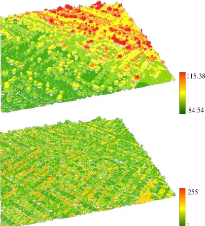
The proposed clustering method was tested on a data subset covering an urban area in Oshawa, Ontario, Canada. The study area includes a variety of land objects such as building roofs, sidewalks, road surface, grass, shrubs, power lines, cars and trees. A flight mission was conducted on September 3rd, 2014 in order to acquire multispectral LiDAR data using the Optech Titan sensor. A subset with a dimension of 490 m by 470 m was clipped for testing, and the LiDAR data are shown in Figure 1.
Figure 1. LiDAR point clouds from C2 colorized by elevation (upper) and intensity (lower)
The Optech Titan sensor acquired the LiDAR data in the three channels from 1075 m flying height with scanning angle of ±20°. The data were collected at 200 kHz/channel PRF and 40 Hz scan frequency. The tested LiDAR data contains about 796226, 825176, and 742158 points from C1, C2, and C3, respectively. Since the 3D reference points are not available, a number of polygons were digitized from an aerial image (Figure 2). Within those polygons, all points were labelled as reference points for the roofs, asphalt and grass classes, while only the canopy points of the trees class were labelled as reference points for the trees class. However, all the understory vegetation or ground points are classified. Table 1 provides the number of reference points for each class with total number of reference points equals to 36421.
Figure 2. Aerial image with the reference polygons
Class Roofs Trees Asphalt Grass
Number of points 111776 12315 5973 6957 Table 1. The number of the reference points
3. METHODOLOGY
The multispectral LiDAR data clustering was applied directly to the 3D point clouds. The LiDAR points from the three channels were first combined and three intensity values for each single LiDAR point were estimated (Morsy et al., 2017b). For any point in C1, the median intensity value from C2, IC2, and C3,
IC3, was estimated using the neighbouring points within a
searching circle of 1 m radius from C2 and C3, respectively. The same applied for C2 and C3, so that each single LiDAR point has six attributes: x, y, z, IC1, IC2and IC3. The LiDAR data
clustering method was then conducted as shown in Figure 3.
Figure 3. The clustering method workflow 255
1 115.38
84.54
3.1 Ground Filtering
The first step in the clustering method is to separate non-ground from ground points. Thus a ground filtering mechanism was applied to the LiDAR points in order to accomplish this step. The points’ elevations were first sorted in ascending order. Then, a statistical analysis – skewness balancing was applied in order to label the higher elevations as non-ground points. The slope of each point with respect to its neighbouring points was then calculated and a threshold value (S_thrd) was applied in
order to label additional non-ground points. In addition, few points with higher elevations were not labelled as non-ground points. Therefore, the remaining points were filtered using a moving circle with radius (r) and height threshold value
(H_thrd) in order to label ground points.
3.2 NDVIs’ Histograms Construction
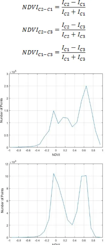
The three raw intensity values IC1, IC2and IC3 were employed to
form three NDVIs, namely NDVIC2-C1, NDVIC2-C3, and NDVI C1-C3, which were defined in Morsy et al. (2016a), for non-ground and ground points as follows:
Figure 4. NDVIC2-C3 histograms constructed from non-ground points (upper) and ground points (lower)
A histogram of each NDVI, which ranges from -1 to1, was constructed with a bin size of 0.1. Figure 4 shows examples of NDVIs’ histograms. Thus, a total of six histograms were constructed (three for non-ground points and three for ground points).
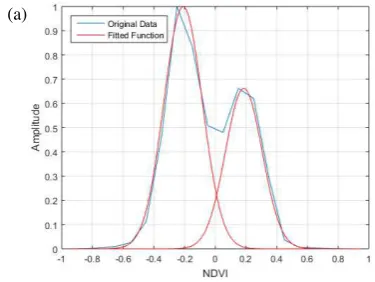
3.3 Gaussian Decomposition
A sum of Gaussian distributions G(x), described by Persson et
al. (2005), was used to fit each NDVI histogram as follows:
Where,
x : the bin value
N : the number of Gaussian components pj : relative weight of the Gaussian (j)
fj(x) : the Gaussian function and defined as:
Where,
j : the mean of Gaussian (j)
σj : the standard deviation of Gaussian (j)
To be able to model the histograms, the parameters N,j and σj
have to be estimated. Since either the non-ground or ground NDVIs’ histograms will be clustered into two classes (i.e., roofs and trees or asphalt and grass), the number of Gaussian components was selected to equal 2 (i.e., N=2). The peak
detection algorithm was used to detect all histograms’ peaks and their locations (i.e., the mean values) (Jutzi and Stilla, 2006). The location of the highest two peaks was then used as the mean values (j) of the two Gaussian components. Based on the
fact that the single Gaussian has two inflection points, the zero crossing of the second derivative was used to obtain the positions of the inflection points of each Gaussian component, and hence the Gaussian’s half width (σj) was calculated (Hofton
et al., 2000).
For each Gaussian component (j), the pj, j and σj were fitted
using the maximum likelihood estimate with Expectation – Maximization (EM) algorithm (Dempster et al., 1977). Following the notation of the EM algorithm described by Persson et al. (2005), the expectation (E) step computes the probability (wij) that each data bin (xi) belongs to Gaussian (j),
starting with that the two Gaussians have equal relative weights (pj), using the following equation:
The maximization (M) step computes the maximum likelihood estimates of the parameters (pj, µj and σj) as follows:
(7) (2)
(3) (1)
(5) (4)
(6)
Where,
yi : the amplitude at bin xi
n: the number of histogram’s bins
The two steps are repeated until convergence or a maximum number of iterations were achieved. The process stops when either (1) the difference between any iteration and the previous iteration is less than 0.001, or (2) the number of iterations is greater than 1000 (Oliver et al., 1996). The quality of the fitted Gaussians of the full waveform LiDAR data has been evaluated using the following formula as defined by Hofton et al. (2000) and Chauve et al. (2007):
Thus, the quality factor ξ should be less than a prescribed accuracy. Similarly, in this paper, the quality of the fitted Gaussians was tested using the aforementioned equation. According to Chauve et al. (2007), a histogram was considered to be well fitted ifξ was less than 0.5. The intersection point of the two adjacent Gaussian components was used as a threshold value (NDVI_thrd) to cluster the LiDAR data of non-ground
and ground histograms into two classes each. If a point had zero intensity value in any two channels, as a result of points’ combination and intensity estimation, this point was labelled as unclassified point.
4. RESULTS AND DISCUSSION
The LiDAR data were clustered into four classes, namely roofs, trees, asphalt and grass. The accuracy assessment was conducted through the creation of confusion matrices, and hence the overall accuracies and kappa statistics were calculated. After the LiDAR points from the three Titan channels were combined, a ground filtering mechanism based on the skewness balancing and the points’ slopes with respect to neighbouring points was applied. Thus, if the point’s slope was greater than a threshold value (S_thrd=10), the point was
labelled as a non-ground point. The consideration of the points’ slopes makes the ground filtering mechanism applicable for not only flat but also sloped terrains. The output ground points were filtered using a moving circle with radius (r=10 m), so if the
height difference was greater than a threshold value (H_thrd=1
m), the point was labelled as a non-ground point and the remaining points were labelled as ground points.
The three NDVIs were subsequently calculated using Equations 1, 2 and 3. NDVIs’ histograms were then constructed and normalized for non-ground and ground points. A sum of two Gaussian distributions was used to model the histograms using EM algorithm. The fitting results of the non-ground and ground histograms are shown in Figure 5 and 6, respectively. The ξ of
Figure 5. Gaussian decomposition of the non-ground NDVIs’ histograms; a) NDVIC2-C1, b) NDVIC2-C3, and c) NDVIC1-C3 (8)
(9)
(10)
(a)
(c)
(a) (b)
Figure 6. Gaussian decomposition of the ground NDVIs’ histograms; a) NDVIC2-C1, b) NDVIC2-C3, and c) NDVIC1-C3
NDVIC2-C1 NDVIC2-C3 NDVIC1-C3
Non-ground 0.34 0.06 0.08
Ground 0.03 0.10 0.15
Table 2. The ξ of the fitted Gaussians
Although the calculated ξ for all fitted Gaussians are less than the prescribed accuracy 0.5, some Gaussians are over-fitted as shown in Figure 5a and Figure 6c, whereas ξ was reduced from 0.34 to 0.08 and from 0.15 to 0.09, respectively when only one Gaussian component was fitted using non-linear least squares. However, in this case, the NDVI_thrd cannot be obtained, and
hence the data cannot be separated into two different classes. Thus, other modelling functions could better fit those histograms as mentioned in (Chauve et al., 2007), such the Lognormal function, where the NDVI_thrd = +σ or the
generalized Gaussian function, where the NDVI_thrd can be
obtained from the intersections of two adjacent components.
4.1 Results Based on Gaussian Decomposition
Table 3 lists the NDVI_thrd obtained from the intersection of
the two Gaussian components for both non-ground and ground histograms. The vegetation (i.e., trees or grass) has high reflectance at C1, C2 and C3. As a result, the calculated NDVIs of the vegetation points exhibited higher values than the built-up areas (i.e., roofs or asphalt). So that, for a particular point, if NDVIC2-C1, NDVIC2-C3 or NDVIC1-C3 ≤ NDVI_thrd, the point was labelled as roofs or asphalt; otherwise, it was labelled as trees or grass. Figure 6 shows the classified point clouds based on the three NDVIs. The confusion matrices and overall accuracies are provided in Table 4, 5 and 6.
Figure 7. Classified LiDAR points based on a) NDVIC2-C1, b) NDVIC2-C3, and c) NDVIC1-C3
NDVIC2-C1 NDVIC2-C3 NDVIC1-C3
Non-ground 0.07 0.43 0.27
Ground 0.01 0.37 0.44
Table 3. Intersection points of Gaussian components (NDVI_thrd)
(a)
(c) (b) (c)
(b)
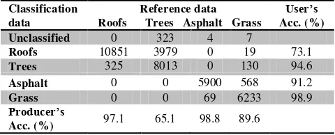
Classification
Overall accuracy: 85.1%, overall Kappa statistic: 0.797.
Table 4. Confusion matrix based on NDVIC2-C1
Classification
Overall accuracy: 95.1%, overall Kappa statistic: 0.933.
Table 5. Confusion matrix based on NDVIC2-C3
Classification Overall accuracy: 79.2%, overall Kappa statistic: 0.715.
Table 6. Confusion matrix based on NDVIC1-C3
As aforementioned the non-ground NDVIC2-C1 histogram (Figure 5a) was over-fitted, which affected the threshold value definition (shifted to the right). As a result, about 34.9% of the tree points were omitted (65.1% producer accuracy), and those points were wrongly classified as roofs. This omission caused a misclassification of the roofs class with about 26.9% (73.1% user accuracy). Similarly, ground NDVIC1-C3 histogram was over-fitted (Figure 6c) and the threshold value was shifted to the right as well. Thus, about 38.6% of the grass points were omitted (61.4% producer accuracy) and mainly classified as asphalt. In addition, about 39.2% (60.8% producer accuracy) of the roofs’ points were wrongly classified as trees when NDVI C1-C3 was used.
Generally, there are three sources of classification errors, including the unclassified class with maximum error of 1.9%, the ground filtering with maximum error of 2.1%, and the NDVIs’ histograms clustering. It should be point out that most of the unclassified non-ground points are power lines. Since the power lines points were only recorded in C1, the intensity values of those points were set to zero in C2 and C3, and hence labelled as unclassified points. This is useful for further extraction of more urban classes.
4.2 Comparison with Previous Studies
Previous studies achieved overall classification accuracies from 85% to 89.5%. The multispectral aerial/satellite imagery was combined with normalized digital surface model derived from LiDAR data (Huang et al., 2008; Chen et al., 2009) or combined with LiDAR height and intensity data (Charaniya et al., 2004; Hartfield et al., 2011; Singh et al., 2012). Compared to previous studies, the presented work in this research used the LiDAR data only and achieved an overall accuracy of 95.1% based on NDVIC2-C3.
Morsy et al. (2017b) used Jenks natural breaks optimization method to cluster the NDVIs histograms of the non-ground and ground points into the same four classes. We applied the same clustering method to the tested dataset in this research for comparison. Table 7 provides the NDVI_thrd values for the
non-ground and ground NDVIs using Jenks breaks optimization. Table 8 shows a comparison between the overall accuracies achieved using Gaussian decomposition, proposed in this research, and Jenks natural breaks optimization method, presented by Morsy et al. (2017b).
NDVIC2-C1 NDVIC2-C3 NDVIC1-C3
Non-ground -0.01 0.32 0.36
Ground -0.02 0.29 0.34
Table 7. NDVI_thrd values obtained from Jenks natural breaks
optimization
Table 8. Comparison of overall accuracies (%)
The achieved overall accuracy based on NDVIC2-C1 and NDVIC2-C3 is very close, while the use of NDVIC1-C3 demonstrated a difference in the overall accuracy of 10.7%. This is mainly because that a significant improvement of roofs and grass detection was achieved using Jenks breaks optimization.
5. CONCLUSIONS
This paper presented a multispectral airborne laser scanning data clustering method for land cover classification of urban areas. The multispectral data were collected by the Optech Titan sensor operating in three channels with wavelengths of 1.550 m, 1.064 m, and 0.532 m. The 3D LiDAR points in the three channels were combined and three intensity values were assigned to each single LiDAR point as a pre-processing step. The clustering method starts with separating non-ground from ground points, followed by NDVIs computation. NDVIs’ histograms were subsequently constructed and each histogram was decomposed into two Gaussian components. The intersection point of the two Gaussian components was then used as a threshold value to cluster non-ground points into roofs and trees, and ground points into asphalt and grass. This method achieved overall accuracies of 85.1%, 95.1%, and 79.2% using NDVIC2-C1, NDVIC2-C3, and NDVIC1-C3, respectively.
The use of Gaussian decomposition succeeds in finding threshold values in order to cluster the NDVIs histograms into
components were over-fitted. As a result, the threshold value definition was affected and caused classification errors. Using other modelling could perform better in fitting the NDVIs histograms and obtaining the threshold values. The presented research work demonstrates the potential use of multispectral LiDAR data in land cover classification. In addition, compared to previous studies, the Gaussian decomposition achieved higher overall accuracy. Further investigations will be devoted to combine the results obtained from the three NDVIs.
ACKNOWLEDGEMENTS
This research work is supported by Discovery Grant from the Natural Sciences and Engineering Research Council of Canada (NSERC) and the Ontario Trillium Scholarship (OTS). The authors would like to thank Dr. Paul E. LaRocque from Teledyne Optech for providing the LiDAR data from the world’s first operational multispectral airborne LiDAR system, the Optech Titan.
REFERENCES
Bakuła, K., Kupidura, P. and Jełowicki, Ł., 2016. Testing of land cover classification from multispectral airborne laser scanning data. ISPRS International Archives of the Photogrammetry, Remote Sensing and Spatial Information Sciences, 41.
Bartels, M., Wei, H. and Mason, D.C., 2006, August. DTM generation from LiDAR data using skewness balancing. In Pattern Recognition, 2006. ICPR 2006. 18th International Conference on (Vol. 1, pp. 566-569). IEEE.
Blomley, R., Jutzi, B. and Weinmann, M., 2016. Classification of airborne laser scanning data using geometric multi-scale features and different neighbourhood types. ISPRS Annals of the Photogrammetry, Remote Sensing and Spatial Information Sciences, Prague, Czech Republic, 3, pp.169-176.
Charaniya, A.P., Manduchi, R. and Lodha, S.K., 2004, June. Supervised parametric classification of aerial LiDAR data. In Computer Vision and Pattern Recognition Workshop, 2004. CVPRW'04. Conference on (pp. 30-30).
Chauve, A., Mallet, C., Bretar, F., Durrieu, S., Deseilligny, M.P. and Puech, W., 2008, July. Processing full-waveform LiDAR data: modelling raw signals. In International archives of photogrammetry, remote sensing and spatial information sciences 2007 (pp. 102-107).
Chen, Y., Su, W., Li, J., Sun, Z., 2009. Hierarchical object oriented classification using very high resolution imagery and LiDAR data over urban areas. Advances in Space Research, 43(7), pp. 1101-1110.
Dempster, A.P., Laird, N.M. and Rubin, D.B., 1977. Maximum likelihood from incomplete data via the EM algorithm. Journal of the royal statistical society. Series B (methodological),
pp.1-38.
Fernandez-Diaz, J.C., Carter, W.E., Glennie, C., Shrestha, R.L., Pan, Z., Ekhtari, N., Singhania, A., Hauser, D. and Sartori, M., 2016. Capability Assessment and Performance Metrics for the Titan Multispectral Mapping LiDAR. Remote Sensing, 8(11),
p.936.
Hartfield, K. A., Landau, K. I., Van Leeuwen, W. J., 2011. Fusion of high resolution aerial multispectral and LiDAR data: Land cover in the context of urban mosquito habitat. Remote Sensing, 3(11), pp. 2364-2383.
Hofton, M.A., Minster, J.B. and Blair, J.B., 2000. Decomposition of laser altimeter waveforms. IEEE Transactions on geoscience and remote sensing, 38(4),
pp.1989-1996.
Huang, H., Brenner, C. and Sester, M., 2013. A generative statistical approach to automatic 3D building roof reconstruction from laser scanning data. ISPRS Journal of photogrammetry and remote sensing, 79, pp.29-43.
Huang, M. J., Shyue, S. W., Lee, L. H., Kao, C. C., 2008. A knowledge-based approach to urban feature classification using aerial imagery with LiDAR data. Photogrammetric Engineering & Remote Sensing, 74(12), pp. 1473-1485.
Jutzi, B. and Stilla, U., 2006. Range determination with waveform recording laser systems using a Wiener Filter. ISPRS Journal of Photogrammetry and Remote Sensing, 61(2),
pp.95-107.
Karila, K., Matikainen, L., Puttonen, E. and Hyyppä, J., 2017. Feasibility of multispectral airborne laser scanning data for road mapping. IEEE Geoscience and Remote Sensing Letters, 14(3),
pp.294-298.
Morsy, S., Shaker, A. and El-Rabbany, A., 2016b. Potential use of multispectral airborne LiDAR data in land cover classification. Proceedings of the Asian conference on Remote Sensing (ACRS), Colombo, Sri Lanka. October 17-21.
Morsy, S., Shaker, A. and El-Rabbany, A., 2017a. Evaluation of distinctive features for land/water classification from multispectral airborne LiDAR data at Lake Ontario.
Proceedings of the 10th International conference on Mobile Mapping Technology (MMT), Cairo, Egypt, May 6-8.
Morsy, S., Shaker, A. and El-Rabbany, A., 2017b. Multispectral LiDAR Data for Land Cover Classification of Urban Areas.
Sensors. 17(5), p.958.
Morsy, S., Shaker, A., El-Rabbany, A. and LaRocque, P.E., 2016a. Airborne multispectral LiDAR data for land-cover classification and land/water mapping using different spectral indexes. ISPRS Annals of the Photogrammetry, Remote Sensing and Spatial Information Sciences, 3(3), pp.217-224.
Nabucet, J., Hubert-Moy, L., Corpetti, T., Launeau, P., Lague, D., Michon, C. and Quenol, H., 2016, October. Evaluation of bispectral LiDAR data for urban vegetation mapping. In SPIE Remote Sensing (pp. 100080I-100080I). International Society
for Optics and Photonics.
Oliver, J.J., Baxter, R.A. and Wallace, C.S., 1996, July. Unsupervised learning using MML. In ICML (pp. 364-372).
Persson, Å., Söderman, U., Töpel, J. and Ahlberg, S., 2005. Visualization and analysis of full-waveform airborne laser scanner data. International Archives of Photogrammetry, Remote Sensing and Spatial Information Sciences, 36(part 3),
p.W19.
Samadzadegan, F., Bigdeli, B. and Ramzi, P., 2010, April. A multiple classifier system for classification of LiDAR remote sensing data using multi-class SVM. In International Workshop on Multiple Classifier Systems (pp. 254-263). Springer Berlin
Heidelberg.
Samadzadegan, F., Hahn, M. and Bigdeli, B., 2009, May. Automatic road extraction from LiDAR data based on classifier fusion. In Urban Remote Sensing Event, 2009 Joint (pp. 1-6).
Singh, K.K., Vogler, J.B., Shoemaker, D.A. and Meentemeyer, R.K., 2012. LiDAR-Landsat data fusion for large-area assessment of urban land cover: Balancing spatial resolution, data volume and mapping accuracy. ISPRS Journal of Photogrammetry and Remote Sensing, 74, pp.110-121.
Xu, S., Vosselman, G. and Elberink, S.O., 2014. Multiple-entity based classification of airborne laser scanning data in urban areas. ISPRS Journal of photogrammetry and remote sensing, 88, pp.1-15.
Yan, W.Y., Shaker, A. and El-Ashmawy, N., 2015. Urban land cover classification using airborne LiDAR data: A review. Remote Sensing of Environment, 158, pp.295-310.
Zhou, L. and Vosselman, G., 2012. Mapping curbstones in airborne and mobile laser scanning data. International Journal of Applied Earth Observation and Geoinformation, 18,
pp.293-304.
Zou, X., Zhao, G., Li, J., Yang, Y. and Fang, Y., 2016. 3D Land Cover Classification Based on Multispectral LiDAR Point Clouds. ISPRS-International Archives of the Photogrammetry, Remote Sensing and Spatial Information Sciences, pp.741-747.