Sensitivity of the SWAT model to the soil and land use data
parametrisation: a case study in the Thyle catchment, Belgium
A.A. Romanowicz
a,∗, M. Vanclooster
a, M. Rounsevell
b, I. La Junesse
baDepartment of Environmental Sciences and Land Use Planning, Universit´e catholique de Louvain,
Croix du Sud 2, BP2, B-1348 Louvain-la-Neuve, Belgium
bDepartment of Geography, Universit´e catholique de Louvain, Place Pasteur 3, B-1348 Louvain-la-Neuve, Belgium
Available online 19 February 2005
Abstract
The sensitivity of the distributed hydrological SWAT model to the pre-processing of soil and land use data was tested for modelling rainfall-runoff processes in the Thyle catchment in Belgium. To analyse this sensitivity, 32 different soil and land use parameterisation scheme were generated and evaluated. The soil input data sources were a generalised soil association map at a scale of 1:500,000, a detailed soil map at a scale of 1:25,000 and the soil profile analytical database AARDEWERK. These soil data were combined with a detailed and a generalised land use map. The results suggest that the SWAT model is extremely sensitive to the quality of the soil and land use data and the adopted pre-processing procedures of the geographically distributed data. The resolution and fragmentation of the original map objects are significantly affected by the internal aggregation procedures of the SWAT model. The catchment size threshold value (CSTV) is thereby a key parameter controlling the internal aggregation procedure in the model. It is shown that a parabolic function characterises the relationship between the CSTV and the hydrological modelling performance of the uncalibrated model, suggesting that optimal uncalibrated modelling results are not obtained when the CSTV is minimised. The hydrological response of the SWAT model to the calculated soil properties is significant. Therefore preference should be given to the calculation of the derived hydrologic soil properties prior to averaging of the profile data. Finally some general guidelines are suggested for parameterising soil and land use in the SWAT model application.
© 2005 Elsevier B.V. All rights reserved.
Keywords: Integrated hydrological modelling; Spatially distributed hydrological models; SWAT; Soil parametrisation; Aggregation
∗
Corresponding author. Tel.: +32 10 47 36 90; fax: +32 10 47 38 33.
E-mail address:[email protected] (A.A. Romanowicz).
1. Introduction
Spatially distributed hydrological models are useful tools to support the design and evaluation of water management plans. A blueprint of this type of model was already presented in the late sixties by Freeze and Harlan (1969)and the current state of the art was recently reviewed byBeven and Feyen (2002). The
spatially distributed nature of these models allows a multi-objective evaluation of the impact of spatially variable forcing terms and catchment properties on the hydrological responses. This property makes spatially distributed hydrological models attractive for the evaluation of land and water management options.
Unfortunately, the use of spatially distributed mod-elling technology in water management decision-making suffers from a series of drawbacks (Abbot and Refsgaard, 1996). First, the data demands for these models is considerable. In many practical cases, data requirements cannot directly be met since the data are simply not available or they do not comply with stan-dard quality targets. Secondly, distributed modelling is exhaustive in terms of computer power and data pro-cessing: advanced geographical information systems (GIS) and computer technology is needed for the ef-ficient processing of data. Finally, there is a lack of scientific understanding of the robustness, sensitivity and validation of these models in relation to different parametrisation schemes (Abbot and Refsgaard, 1996). In particular, questions are raised about the appropri-ate resolution of the spatially distributed input data. As it has already been proven in numerous studies (e.g.
Becker and Braun, 1999), the resolution and the aggre-gation of the GIS data have a considerable impact on the modelling of the rainfall runoff processes. There-fore the parametrisation of the soil, the vegetation and the climate should be analysed in detail for different distributed hydrological modelling types and different hydrological catchments, and this prior to any mod-elling calibration (Refsgaard et al., 1996).
To contribute to this last challenge, this paper presents an analysis of the sensitivity of the distributed hydrological model soil and water assessment tool (SWAT, Arnold et al., 1993) to the soil and land
use parametrisation for simulating rainfall-runoff pro-cesses in a small agricultural catchment in the central part of Belgium. The SWAT model was considered in this study since it is an integrated hydrological model that simulates both the qualitative as well as quantita-tive terms of hydrological balances (Fig. 1). Integrated hydrological models are nowadays needed to support the implementation of integrated water management plans and to comply with the current requirements of the European Water Directive. In addition, the SWAT model is interfaced with the ARC-VIEWTMsoftware which allows easy pre-and post processing of the spa-tially distributed input data, driving the rainfall-runoff process. Finally, the SWAT model is a spatially dis-tributed hydrological model, which means that the im-pact of spatially variable input parameter changes such as land use change can easily be modelled. The model is well documented, transparent and the source code is directly downloadable from the web page at no cost. The software is supported by the knowledge of its de-veloper and users by means of an e-mailing list server and a discussion forum on the web page. It is therefore a hydrological model which respects the principles of good modelling practice (STOWA, 1999). Finally, the validation status of this code is known, and continuous to be developed (e.g.Conan et al., 2002).
An evaluation is made of the prepared available soil and land use data for the SWAT model and how the internal aggregation procedures affect the simulation of the rainfall-runoff processes. The SWAT model is a physically based model and includes therefore a phys-ical description of the soil water balance, which means that the soil parameterisation is one of the main param-eters during the modelling process. Previous studies (e.g.Muttiah and Wurbs, 2002) have shown that the SWAT model is sensitive to its soil parameterisation,
in particular to available water capacity. Yet, in these studies, the sensitivity of the soil parameterisation was investigated for catchments in the United States and the conclusions were conditional to the considered land use and surface topography parameterisation. In the case of other catchments where different land use and topographical pre-processing is considered, this may give different results (Chess Project, 2001). Specific attention is also paid to the spatial resolution of soil data and the interaction of the soil data parameterisa-tion with the modelling of the land use and surface topography. In practice, SWAT simulates the rainfall-runoff process at the sub-catchment level by deriving hydrological response units (HRUs). Up-scaling of the spatially distributed soil and land use maps takes place during the creation of the HRUs and the result of this up-scaling will depend therefore on the initial resolu-tion considered for these data and will affect the simu-lated rainfall-runoff process.
2. Materials and methods
2.1. Model description
The SWAT model (Arnold et al., 1993) was de-veloped to predict the impact of land management practices on water, sediment and agricultural chemical yields in large complex catchments with different soil, land use and management conditions over long periods of time. It is a physically based, continuous model. In this study, only the hydrological and climate compo-nent of the SWAT modelling system was considered. Use was made of the AV-SWAT version of the model (an integrated version within ArcViewTM), which has been fully documented byNeitsch et al. (2001)and is available athttp://www.brc.tamus.edu/swat/(access in November 2001). Only the parts of the model that are relevant to this case study are presented in the below description.
In AV-SWAT, the pre-processing of the data is done by applying some of the ArcViewTM GIS functions. This involves the creation of the river network, the catchment area, and the sub-catchments. The latter step is crucial, since it creates the boundaries for the further simulation. The definition of the sub-catchment size is based on the threshold value (CSTV) which is defined by the user. This value is also the basis for the definition
of the hydrological response units (HRUs), which also involves aggregation of the input data (FitzHugh and Mackay, 2000). The threshold value for the catchment size is selected by the model user from a series of pre-defined relative CSTVs pre-defined by the developer (the absolute value depends on the total catchment size). Possible relative threshold values are (i) the smallest size, implying a low aggregation level of input data, (ii) the suggested value size by the model developer, implying that the modelling depends more on the com-putational time and the size of the catchment, (iii) an intermediate value, implying an intermediate aggrega-tion level; and (iv) the maximum value, implying a high aggregation level. Since hydrological attributes are defined at the sub-catchment level, precaution is needed when defining the CSTV. After the definition of the CSTV, SWAT disaggregates heteorogenous catch-ments into sub-catchcatch-ments and homogeneous HRUs. Hydrological attributes are assigned at the HRU level by considering either multiple or dominant attributes of the underlying spatially distributed input attributes. In this case study, only the dominant input attribute option was considered. The HRU is also the reference unit for which the hydrological balance is calculated. Total catchment balance terms are obtained by aggre-gating the results of each HRU calculation. The use of the HRU concept allows consideration of spatially distributed catchment properties in a computationally efficient way and has been used in different hydrolog-ical models (e.g.Becker and Braun, 1999).
2.2. The catchment area
The study focused on the modelling of the rainfall-runoff processes at the outlet of a catchment and its sensitivity to different discretisation procedures. The gauging station of the catchment outlet is situated at Suzeri and daily measurements are available from the early 1970s. The outflow data are collected by R´egion Wallonne (DGRNE-SCENN). Data were used for the year 1999.
2.3. General input data
It is well known that the quality of the DEM will have a strong influence on the final output of the hydro-logical model (Defourny et al., 1999). We used there-fore the finest resolution DEM available for the study area. The DEM map used was created by the local gov-ernment authorities and was used in previous studies for the Dyle catchment (Persoons, 1999). The weather data for 1999 were obtained from the Belgian Royal Meteo-rological Institute (KMI-IRM). These data include the daily precipitation rate, the daily maximum/minimum temperature, the mean monthly values of wind speed, and solar radiation. Data from five precipitation tions with daily measurements were used. Three sta-tions were used to characterize the minimum and max-imum temperatures. All the data were validated by the standard procedures used by the IRM. The selected stations are located either within the Thyle catchment itself or within the upper catchment of the Dyle river.
The 1999 land use map was created using the SIGEC data set, combined with LandsatTM satellite images and the IGN topographical map 1/50,000. The SIGEC data set includes information about the crop distribu-tion over the catchment area and is based on the claims of the farmers for the EU subsidies. A standard clas-sification has resulted in 50 types of land use within the study area, which includes, inter alia, all types of agriculture crops. The SWAT data set consist of much less land use types. Additionally to that those of the land use types which were representing the area in less then 1% would not be taken into consideration while modelling with SWAT. Therefore, the detailed SIGEC land use data classes were generalised to 23 land use types, later called detailed land use map. Those of the agriculture practice which were represented in small percentage where summarised as generic agriculture. To evaluate the impact of the aggregation of the land use on the hydrological modelling performance, a
gen-eralised 5 classes land use map was defined from the 23 classes land use map. Where all agricultural crops are summarised as ‘agriculture’, two forests types are represented by one mixed forest, and one class also represents two urban classes of detail land use map. In the subsequent discussion reference will be made to the generalised land use map of 5 classes.
Two different soil maps were used: (i) a soil asso-ciation map, which is available at a scale of 1:500,000 (Comit´e National de G´eographie, 1970) referred to as the generalised soil map; and (ii) a detailed soil map (maps: 129◦E, 130◦W, 142◦E, and 143◦W), which is available at a scale of 1:25,000 (IRSIA, 1972). The as-sociation map has 39 different soil asas-sociations for Bel-gium (Van Orshoven and Vandenbroucke, 1993a). The study catchment is characterised by three associations and 60 detailed soil map units. To parameterise the soil map units of the two different soil maps, use was made of the Belgian analytical soil database AARDEWERK (Van Orshoven, 1993b). This analytical database was matched with the different soil mapping units of the two soil maps. For the generalised map, all the soil profiles that were located within one of the three asso-ciations were extracted and stored in a file considering a pure class matching procedure. For the detailed soil map, however, soil profiles could not be matched to all the 60 mapping units. Therefore, the detailed soil map was aggregated to result in a new six class soil map and then the available profiles where connected to the new obtained soil units. The aggregation was done by combining soils to there higher level, in terms of the soil taxonomic groupings for Belgian soils. For each of the new mapping units, soil profiles were extracted, resulting in 87 profiles and 716 horizon descriptions.
2.3.1. Soil parameterisation
den-sity, available water capacity, soil organic matter) use was made of the pedotransfer rules described below.
The organic matter (MO) content was calculated from the equation (Van Orshoven, 1993b):
MO=percentage of carbon×1.7924 (1)
The bulk density (BD) was calculated using the pedo-transfer function ofAdams (1973), later on developed byVan Orshoven (1993b)
where MO is the percentage of organic matter;ρMO the density of organic matter = 0.224 g/cm3;ρMMthe density of mineral matter according to the texture class (class Z,S-sand: 1.55 g/cm3; class P,A,E-sandy-loamy: 1.41 g/cm3; class L-loamy:1.3 g/cm3; class U-clay: 1.35 g/cm3).
In order to calculate the hydraulic conductivity (Ksat) and the available water capacity (AWC), pedo-transfer functions from the HYPRESS database were used (Woesten et al., 1998).
Different averaging procedures were used to derive soil attributes at the mapping unit level. The ensem-ble of basic soil data per mapping unit was averaged to yield a single mean value of the basic properties (for the same soil type) for the considered mapping unit prior to the calculation of the derived property. Alternatively, the derived properties were first calculated for each single profile after which a single value for a mapping
unit was obtained by averaging the set of derived prop-erties. The chain of calculations can be summarised by the following logical sequence:
1. PM on the detailed map→CDP→CMDP→SWAT,
2. PM on the detailed map→CMBP→CDP→SWAT,
3. PM on the generic map→CDP−CMDP→SWAT,
4. PM on the generic map→CMBP→CDP→SWAT
with PM, profile matching; CDP, calculate derived properties; CMDP, calculate mean derived properties; CMBP, calculate mean basic properties.
2.3.2. Modelling
Four values for the CSTV were considered in the scenario-analysis: sub-catchment size corresponding to the maximum area, i.e. one catchment; sub-catchment size suggested by the model developer, i.e. based on the total size of the considered catchment, re-sulting in 27 sub-catchments of size below 100 ha; a CSTV of 60 ha, resulting in 47 sub-catchments; and fi-nally a CSTV of 20 ha resulting in 145 sub-catchments. Lower threshold values were not possible due to com-putational limitations.
The combination of the two soil maps, with two land use maps, two soil analytical data averaging schemes, and four CSTVs resulted in a total of 32 different schemes for modelling. To characterize the soil type
Table 1
Map indicators used to compare the basic input map and the generic derived map
Symbol Definition of map indicator Calculation procedure
G1 Number of cells of classxthat after aggregation correspond to the original map ArcView
G2 Number of cells assumed to be a different class ArcView
G3 Number of original cells not used for simulation ArcView
G4 Total cells per classxgenerated by the SWAT model ArcView
G5 Original number of cells per classx ArcView
NP Number of patches (extent of subdivision or fragmentation of the patches) Fragstat PD Number of patches on a per area unit basis (value in hectares) Fragstat Area-Min Patch area distribution the smaller the size the more fragmented the map is, value in hectares
PR Number of patches within the landscape Fragstat
PRD Number of different patch types presented within the landscape (value in hectares) Fragstat RPR Number of different patch types presented within the landscape boundary divided by the
maxi-mum potential number of patch types in the original data (value in percentage)—used only for the comparison
Fragstat
Table 2
The hydrological evaluation indices
Definition Reference Comments
CNS=1−
(Oi−Pi)2
(Oi−O¯)2 Nash–Sutcliffe (Nash and Sutcliffe, 1970) The optimal statistical value occurs when the
value does reach 1 AE=
n
i=1
Pi−Oi
n Average error (Jannsen and Heuberger, 1995) The optimal statistical value is close to 0
RMSE=
n
i=1 (Pi−Oi)2
n
×100 Root mean square error (Jannsen and Heuberger, 1995) In %; the optimal statistical value is close to 0
RMS=
n
i=1 (Pi−Oi)2
n
×100 Root mean square (Loague and Green, 1991) In %; the optimal statistical value is close to 0
CRM=
n
i=1Oi−
n
i=1Pi
n
i=1Oi
Coefficient of residual mass (Loague and Green, 1991) This indicator identifies when the model over es-timates (negative values) or undereses-timates (pos-itive values) the values
Oi, observed value; ¯O, mean observed value;Pi, simulated value.
and land use within each HRU, the dominant soil and land use was considered (here dominant means the type which covers the area in majority). All other SWAT pa-rameters were given their default values, and no cali-bration was performed.
2.4. Model evaluation
2.4.1. Evaluation of the pre-processing
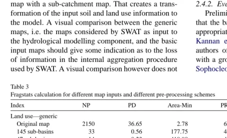
The modeller does not have any influence on how the HRU is attributed. The attribution are internally defined by overlaying the input soil map and land use map with a sub-catchment map. That creates a trans-formation of the input soil and land use intrans-formation to the model. A visual comparison between the generic maps, i.e. the maps considered by SWAT as input to the hydrological modelling component, and the basic input maps should give some indication as to the loss of information in the internal aggregation procedure used by SWAT. A visual comparison however does not
allow to elucidate the differences in a synthetic way. Therefore the visual comparison was completed with the calculation of five map indicators in ArcViewTM and seven map indicators using FRAGSTATS (http://www.umass.edu/landeco/research/fragstats/ fragstats.html, access in August 2002) (McGarigal et al., 2002). The latter tool is a public domain software program designed to compute a wide variety of land-scape metrics the emphasis on the spatial distribution of map patterns. The map indicators are defined in
Table 1.
2.4.2. Evaluation of the hydrological modelling
Preliminary results with the SWAT model showed that the baseflow component in the catchment is not appropriately modelled. This was also observed by
Kannan et al. (2002). To solve this problem, the authors of the model recommend to couple SWAT with a groundwater flow model as illustrated e.g. by
Sophocleous and Perkins, 2000. The use of this
cou-Table 3
Fragstats calculation for different map inputs and different pre-processing schemes
Index NP PD Area-Min PR PRD RPR AI
Land use—generic
Original map 2150 36.65 2.78 6 0.1023 – 80.18
145 sub-basins 33 0.56 177.75 4 0.0682 66.67 97.46
47 sub-basins 14 0.23 418.98 4 0.0682 66.67 98.48
27 sub-basins 8 0.14 733.21 4 0.0682 66.67 98.92
1 sub-basin 1 0.02 5865.72 1 0.017 16.67 99.73
Land use—detail
Original map 5141 87.64 1.14 23 0.39 – 68.8
145 sub-basins 48 0.82 122.2 12 0.20 52.17 96.85
47 sub-basins 15 0.26 391 7 0.12 30.43 98.4
27 sub-basins 14 0.24 418.98 6 0.10 26.09 98.83
1 sub-basin 1 0.02 5865.72 1 0.017 4.35 99.73
Soil map—generic
Original map 28 0.48 209.49 3 0.05 – 97.60
145 sub-basins 15 0.26 391 3 0.05 100 97.77
47 sub-basins 10 0.17 586.57 3 0.5 100 98.47
27 sub-basins 7 0.12 837.96 3 0.5 100 98.87
1 sub-basin 1 0.02 5865.72 1 0.017 33.33 99.73
Soil map—detail
Original map 1159 18.84 5.31 6 0.1 – 82.21
145 sub-basins 29 0.49 202.27 6 0.1 50 97.3
47 sub-basins 8 0.14 733.2 3 0.05 50 98.79
27 sub-basins 8 0.14 733.2 3 0.05 50 98.79
1 sub-basin 1 0.02 5865.72 1 0.017 16.67 99.73
pled version, however, was not possible in this study, since the code is not publicly available. An alternative approach is to use the SWAT model to simulate only the surface and interflow component of the hydrological cycle. This can be implemented by separating the base flow component from the surface flow component in the observed hydrograph data by means of automated separation techniques (Arnold and Allen, 1999) and comparing modelled surface flow with estimated sur-face flow. In this paper, the hydrograph recession curve displacement method was used as presented byArnold and Allen (1999)andArnold et al. (1995). This is an au-tomated digital filter program based on the Rorabaugh hydrograph recession curve displacement method us-ing daily stream flow. The method was later extended and tested in the work ofNathan and McMahon (1990)
andRutledge and Daniel (1994)and is called the au-tomated master recession curve method. The equation of the filter yields:
qt=βqt−1+ (1+β)
2 (Qt−Qt−1) (3)
whereqt is a filtered surface runoff at the time stept;
Qtthe original stream flow; andβthe filter parameter
provided by the SWAT model developer. The base flow (B) is calculated with the equation:
Bt =Qt−qt (4)
The modelled peak flow for the different modelling schemes were compared with the peak flow measured at the Suzeri outlet of the Thyle catchment for the year 1999. Graphical comparison of simulated ver-sus measured outflow was combined with statistical modelling performance indicators to assess the mod-elling performance. The modmod-elling performance was calculated by using a set of different modelling eval-uation indicators. The definition of the different indi-cators is given inTable 2. It has to be added that be-cause the initial conditions of the modelling have to be stabilised therefore the model have been ran for 2 years but only the second year is taken into conside-ration.
3. Results and discussion
3.1. Evaluation of the generic land use and soil map
The land use maps generated by the SWAT model using the generic land use map as an input to the hydrological simulation are given inFig. 2. The impact of the CSTV on the generic land use map is marked. The geometry of the patches of land use classes changes significantly, as do the total area and the shape of the land use class patches. In addition, some land use classes disappear in the aggregation procedure. The change of shape of the land use class patches is of concern for hydrological modelling. Compared with the generic land use map, land use class patches are much more dispersed throughout the catchment
and that affects significantly the fast response of the catchment to intense rainfall.
A quantitative comparison of the original and generic land use maps using the performance indicators ofTable 1is given inTable 3andFig. 3a. Because the model with different classes as well as four sizes of the sub-catchment generated four maps, only the results for a single land use class are presented (the pasture class).
As might be expected, the aggregation procedure used to derive the generic maps resulted in a consider-able loss of information. The change in the distribution of the land use class patches and the disappearance of some of the land use classes in the generic map is illustrated by the decrease of parameters (NP, PD, PR and RPR) when the number of sub-catchments de-creases. As can be seen, the number of patches in the
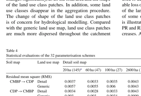
Table 4
Statistical evaluations of the 32 parameterisation schemes
Soil map Land use map Detail soil map Generic soil map
20 ha (145)a 60 ha (47) 100 ha (27) 2600 ha (1) 20 ha (145) 60 ha (47) 100 ha (27) 2600 ha (1) Residual mean square (RMS)
CMBP→CDP Detail 0.0037 0.0033 0.0035 0.0043 0.006 0.053 0.006 0.012 Generic 0.0057 0.0055 0.006 0.0043 0.008 0.008 0.009 0.015 CDP→CMBP Detail 0.0034 0.0028 0.0033 0.0043 0.004 0.004 0.005 0.011 Generic 0.003 0.003 0.0034 0.0009 0.006 0.006 0.007 0.014 Root mean square error (RMSE)
CMBP→CDP Detail 7.04 6.268 6.744 8.279 10.74 10.068 10.96 21.823 Generic 10.793 10.4 11.091 18.009 14.953 15.223 16.564 27.92 CDP→CMBP Detail 6.46 5.326 6.255 8.185 8.005 7.683 8.506 20.157
Generic 5.898 5.701 6.475 8.152 11.695 12.064 13.626 27.262 Average error (AE)
CMBP→CDP Detail −0.0122 −0.0148 −0.019 −0.0337 0.003 0.0046 0.008 0.035 Generic −0.011 −0.013 −0.017 −0.026 0.004 0.006 −0.008 0.037 CDP→CMBP Detail −0.004 −0.0048 −0.0037 0.0037 −0.002 −0.0008 0.0025 0.032 Generic −0.007 −0.0054 −0.004 0.0036 −0.0013 0.0008 0.003 0.034 Coefficient of residual mass (CRM)
CMBP→CDP Detail 0.23 0.28 0.36 0.64 −0.063 −0.087 −0.146 −0.66 Generic 0.2087 0.251 0.33 0.486 −0.080 −0.114 −0.159 −0.711 CDP→CMBP Detail 0.085 0.0908 0.07 −0.07 0.046 0.015 −0.047 −0.597 Generic 0.126 0.1022 0.079 −0.068 0.025 −0.015 −0.063 −0.647 Nash–Sutcliffe coefficient (CNS)
CMBP→CDP Detail 0.31 0.386 0.339 0.189 −0.052 0.0138 −0.07 −1.137 Generic −0.057 −0.0189 −0.086 −0.764 −0.465 −0.491 −0.622 −1.735 CDP→CMBP Detail 0.367 0.478 0.387 0.198 0.216 0.247 0.167 −0.974 Generic 0.422 0.442 0.366 0.202 −0.1455 −0.182 −0.33 −1.67 CDP, calculate derived properties; CMBP, calculate mean basic properties.
generic map decreases rapidly and some of the classes in certain combinations were not used, despite covering the area substantially in absolute terms (Fig. 3b). This means that, when patches of a certain class are widely dispersed, the model may not consider this class. It should also be noted that the degree to which the orig-inal map is fragmented is very high. The comparison index (RPR) confirms that most of the information is
not used by the model. From the aggregation index (AI) it can be concluded that the data are aggregated to a very high level.
When analysing the number of grid indicators in terms of CSTVs a similar pattern can be observed as in the example inFig. 3a. The number of grids in the generic map classified as the truth-value on the original map increases with an increase in the number of
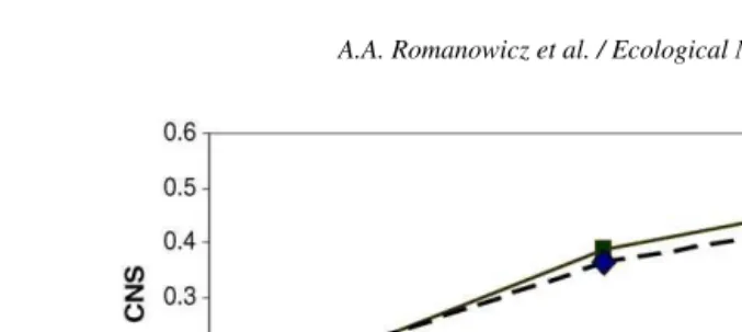
Fig. 5. The Nash–Sutcliffe coefficient for different map inputs combination and different amount of sub-catchments (the CDP→CMBP calculation).
catchments. For the pasture land use class the number of grids aggregated as pasture decreases. This can be explained by the spatial dispersion of pasture patches in the original map. Assigning the dominant land use to a sub-catchment unit will result in the disappearance of dispersed land use classes when aggregation takes place.
Similar conclusions can be drawn from the analysis of the properties of the generic soil map in relation to the original soil map.
Hence, it is evident that the internal aggregation pro-duced within SWAT, driven by the CSTV, will have sig-nificant effects on the generic land use and soil maps. Even if the original detailed land use and soil maps were used, considerable information would have been lost in the internal aggregation, if high CSTVs were used. Users of the model should therefore be aware of the impact of this threshold value on land use and soil maps and evaluate the consequences of this for the performance of the hydrological model. Reduc-ing the CSTV to represent correctly the fragmenta-tion of the original map on the derived map is not possible from a computational point of view. There-fore, we propose an external aggregation of the soil and land use map that is compatible with the CSTV imposed by the SWAT model. By doing so, the user will have greater influence on what is happening during the pre-processing, and this will ensure that the maps are aggregated for the HRUs values in a more realistic way.
3.2. Evaluation of the hydrological modelling
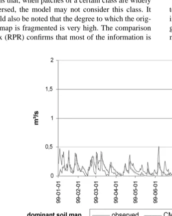
The impact of the different aggregation and soil parameterisation procedures on the predicted rainfall-runoff is illustrated inTable 4andFig. 4. It must be emphasised that the model was not calibrated and so, the performance indices are not high. However given the uncertainty due to the input data (e.g. rainfall data, discharge measurements) the results with the uncali-brated SWAT model were satisfactory.
In most cases, the simulation model underestimates the observed values, which is in agreement with the study ofChanasyk et al. (2002). The indices inTable 4
suggest that with an increase in the sub-catchment num-ber the statistical performance of the model increases to a certain point. After reaching this point increasing the number of sub-basins will create a poor represen-tation of the catchment leading to decreases in model performance. The use of the pedotransfer function (ptf) prior to averaging reflects more precisely each of the soil properties in mathematical terms, and as hypoth-esized this procedure gave better results then the use of ptf after averaging the basic properties. Thus, the soil component of the SWAT model is very sensitive and proper preparation of available data for the case study is advisable. The difference created by the two soil property calculations is represented by an example inFig. 4.
the number of sub-catchments is not linearly propor-tional to the modelling performance.Fig. 5illustrates that the optimal CNS index is obtained with 47 sub-catchments. This means there is an optimal value for CSTV beyond which the model improvement will de-crease. However, the value of 60% of the CSTV ‘sug-gested by the developer’ is probably the optimal value for the catchment size when using a similar set up. The major reason for observing a decrease in model performance could be because of the input maps (soil and land use) which were used with the ArcView in-terface. A decrease in the number of sub-basins will create an artificial soil and land use combination and so it is advisable to use the multiple HRU distribution with a considerably larger CSTV than a smaller value for CSTV and a dominant HRU distribution.
4. Conclusion
This study has shown that the SWAT model is very sensitive to the internal and external pre-processing of the soil and land use data. Consequently, the in-put data resolution and classification should be trans-formed prior to the hydrological modelling itself by the internal aggregation procedure. Care should be taken, therefore, to see how the model pre-processes the soil and land use input data and to which degree some of the input transformations affect the model outputs. The threshold value for the sub-catchment size is a critical parameter in the SWAT model, driving the internal ag-gregation and therefore its impacts on modelling per-formance.
The simulated hydrographs at the outlet of a rural catchment in the central part of Belgium were strongly influenced by the soil parameterisation scheme. With GIS technology, soil map information can easily be included within distributed hydrological models. Yet, the parameterisation procedures from readily available data should be evaluated carefully. The modelling per-formance analysis suggested that derived soil prop-erties should be calculated directly on the basic soil data, prior to averaging. In terms of using the AVSWAT model, the user should analyse the input maps and pre-pare them prior to using the model. This will provide a more reliable overlay of the land use and soil map for the application of the hydrological model.
The work presented here also raises concerns that are relevant to a broader community of people (sci-entists and water authorities). The implementation of the Water Framework Directive in Europe requires the application of different hydrological models with GIS technology. As this work has shown a good understand-ing is needed of not only hydrological models but also of the GIS procedures for data input. This implies the need for a methodology of model application which will be understandable to all users. Thus special atten-tion needs to be given to the ways in which GIS data are created, manipulated and transformed by the ap-plied model. Special attention should be paid to the pre-processing of data for which the model user has no, or very little, influence.
Acknowledgements
This study is supported by the Fifth Framework Programme of the European Communities, the Di-rectorate General Research and the Energy, Environ-ment and Sustainable DevelopEnviron-ment Programme. The authors would like to acknowledge the developers of the AvSwat interface.
References
Abbot, B.M., Refsgaard, J.Ch., 1996. Distributed Hydrological Mod-elling. Kluwer Academic Publishers, 321 pp.
Adams, W.A., 1973. The effect of organic matter on the bulk and true densities of some uncultivated podsolic soils. Soil Sci. 24, 10–17.
Arnold, J.G., Engel, B.A., Srinivasan, R., 1993. Continuous-time, grid cell watershed model. In: Proceedings of the Conference, Spokane, WA, June 18–19, pp. 267–278.
Arnold, J.G., Allen, P.M., Muttiah, R., Bernhardt, G., 1995. Auto-mated base flow separation and recession analysis techniques. Groundwater 33 (6), 1010–1018.
Arnold, J.G., Allen, P.M., 1999. Automated methods for estimating baseflow and ground water recharge from streamflow records. J. Am. Water Resour. Assoc. 35 (2), 411–424.
Becker, A., Braun, P., 1999. Disaggregation, aggregation and spatial scaling in hydrological modelling. J. Hydrol. 217, 239–252. Beven, K., Feyen, J., 2002. The Future of Distributed Modelling,
Hydrological Processes, vol. 16, Willy, No. 2, p. 1.
Chess Project, 2001. Climate, hydrochemistry and economics of surface-water systems. Summary of the Chess project, Re-port July 2001. Final reRe-port:http://www.nwl.ac.uk/ih/research/ iresearch.html.
Comit´e National de G´eographie, 1970. Carte p´edologique (d’association des soil) de la Belgique ou 1:500 000.
Conan, C., Bouraoui, F., de Marsily, G., Bidoglio, G., 2002. A mod-elling of the water quality in the Coet-Dan catchment (France). In: Proceedings from the Third International Conference on Wa-ter Resources and Environment Research, vol. II, Dresden, Ger-many, pp. 222–226.
Defourny, P., Hecquet, G., Philippart, T., 1999. In: Lowell, K., Ja-ton, A. (Eds.), Digital Terrain Modeling: Accuracy Assessment and Hydrological Simulation Sensitivity, Published in Spatial Accuracy Assessment: Land information Uncertainty in Natural Resources. Ann Arbor Press, Chelsea, Michigan, p. 323. FitzHugh, T.W., Mackay, D.S., 2000. Impacts of input parameter
spatial aggregation on an agricultural nonpoint source pollution model. J. Hydrol. 236, 35–53.
Freeze, R.A., Harlan, R.L., 1969. Blueprint for a physically-based digitally-simulated hydrological response model. J. Hydrol. 9, 237–258.
IRSIA, 1972. Institut pour l’encouragement de la Recherche Scien-tifique dans l’Industrie l’Agriculture, maped issued by Institut G´eographique Militaire in 1972. Survey taken in 1958. Jannsen, P.H.M., Heuberger, P.S.C., 1995. Calibration of
process-oriented models. Ecol. Modell. 83, 55–66.
Kannan, N., White, S.M., Worrall, F., Groves, S., 2002. Hydrologi-cal modelling of small catchments using SWAT. In: Proceedings of the XXVII Conference on General Assembly, Nice, France, April, 21–26. European Geophysical Society.
Loague, K., Green, R.E., 1991. Statistical and graphical methods for evaluating solute transport models: overview and application. J. Contam. Hydrol. 7, 51–73.
McGarigal, K., Cushman, S.A., Neel, M.C., Ene, E., 2002. FRAGSTATS: Spatial Pattern Analysis Program for Categori-cal Maps. Computer software program produced by the authors at the University of Massachusetts, Amherst.
Muttiah, R.S., Wurbs, R.A., 2002. Scale-dependent soil and cli-mate variability effects on watershed water balance of the SWAT model. J. Hydrol. 256, 264–285.
Nash, J.E., Sutcliffe, J.E., 1970. River flow forecasting through con-ceptual models. Part I. A discussion of principles. J. Hydrol. 10 (3), 282–290.
Nathan, R.J., McMahon, T.A., 1990. Evaluation of automated tech-niques method for base flow and recession analyses. Water Re-sour. Res. 26 (7), 1465–1473.
Neitsch, S.L., Arnold, J.G., Kiniry, J.R., Williams, J.R., 2001. Soil and Water Assessment Tool. Theoretical Documentation and User’s Manual. Version 2000. USDA-ARS, Temple, TX, USA, 506 pp.
Persoons, E., 1999.Bassin versant de la Dyle en R´egion wallonne—Crues de projet (pour des p´eriodes de retour de 1/20-1/50-1/100 ans). Internal document.
Refsgaard, J.Ch., Storm, B., 1996. Construction, calibration and vali-dation of hydrological models. In: Abbot, B.M., Refsgaard, J.Ch. (Eds.), Distributed Hydrological Modelling. Kluwer Academic Publishers, p. 321.
Rutledge, A.T., Daniel, C.C., 1994. Testing an automated method to estimate ground-water recharge from streamflow records. Groundwater 32 (2), 180–189.
Sophocleous, M., Perkins, S.P., 2000. Methodology and application of combined watershed and ground-water models in Kansas. J. Hydrol. 236, 185–201.
STOWA, 1999. STOWA Report 99-05. Good Modelling Practice handbook, 122 pp.
Van Orshoven, J., Vandenbroucke, D., 1993a. Guide de l’utilisateur de Aardewerk base de donn´ees de profils p´edologiques, Novem-ber 1993 Rapport 18B, Katholieke Universiteit Leuven, 40 pp. Van Orshoven, J., 1993b. Assessing hydrodynamic land qualities
from the soil survey data. Th`ese de doctorat. Katholiek Univer-siteit Leuven, 263 pp.