User JOEWA:Job EFF01427:6264_ch11:Pg 281:25874#/eps at 100%
*25874*
Wed, Feb 13, 2002 10:26 AM In Chapter 10 we assembled the pieces of the IS–LMmodel.We saw that the IScurve represents the equilibrium in the market for goods and services, that the LMcurve represents the equilibrium in the market for real money balances, and that the ISand LMcurves together determine the interest rate and national in-come in the short run when the price level is fixed. Now we turn our attention to applying the IS–LMmodel to analyze three issues.
First, we examine the potential causes of fluctuations in national income. We use the IS–LM model to see how changes in the exogenous variables (govern-ment purchases, taxes, and the money supply) influence the endogenous variables (the interest rate and national income). We also examine how various shocks to the goods markets (the IS curve) and the money market (the LMcurve) affect the interest rate and national income in the short run.
Second, we discuss how the IS–LM model fits into the model of aggregate supply and aggregate demand we introduced in Chapter 9. In particular, we ex-amine how the IS–LMmodel provides a theory of the slope and position of the aggregate demand curve. Here we relax the assumption that the price level is fixed, and we show that the IS–LM model implies a negative relationship be-tween the price level and national income. The model can also tell us what events shift the aggregate demand curve and in what direction.
Third, we examine the Great Depression of the 1930s. As this chapter’s open-ing quotation indicates, this episode gave birth to short-run macroeconomic the-ory, for it led Keynes and his many followers to think that aggregate demand was the key to understanding fluctuations in national income. With the benefit of hindsight, we can use the IS–LMmodel to discuss the various explanations of this traumatic economic downturn.
| 281
11
Aggregate Demand II
C H A P T E RScience is a parasite: the greater the patient population the better the
ad-vance in physiology and pathology; and out of pathology arises therapy.
The year 1932 was the trough of the great depression, and from its rotten
soil was belatedly begot a new subject that today we call macroeconomics.
11-1
Explaining Fluctuations With
the
IS
–
LM
Model
The intersection of the IS curve and the LMcurve determines the level of na-tional income.When one of these curves shifts, the short-run equilibrium of the economy changes, and national income fluctuates. In this section we examine how changes in policy and shocks to the economy can cause these curves to shift.
How Fiscal Policy Shifts the
IS
Curve and
Changes the Short-Run Equilibrium
We begin by examining how changes in fiscal policy (government purchases and taxes) alter the economy’s short-run equilibrium. Recall that changes in fiscal policy influence planned expenditure and thereby shift the IScurve.The IS–LM model shows how these shifts in the IScurve affect income and the interest rate. Changes in Government Purchases Consider an increase in government pur-chases of
D
G.The government-purchases multiplier in the Keynesian cross tells us that, at any given interest rate, this change in fiscal policy raises the level of income byD
G/(1 −MPC).Therefore, as Figure 11-1 shows, the IScurve shifts to the right by this amount.The equilibrium of the economy moves from point A to point B. The increase in government purchases raises both income and the interest rate.To understand fully what’s happening in Figure 11-1, it helps to keep in mind the building blocks for the IS–LMmodel from the preceding chapter—the Keynesian cross and the theory of liquidity preference. Here is the story. When the government 282| P A R T I V Business Cycle Theory: The Economy in the Short Run
f i g u r e 1 1 - 1
Interest rate, r
Income, output,Y
Y1 Y2
r1 r2
IS1 B
A IS
2 LM
2. . . . which raises income . . . 3. . . . and the interest rate.
1. The IS curve shifts to the right by ⌬G/(1 ⫺MPC), . . .
An Increase in Government Purchases in the IS–LMModel An increase in government purchases shifts the IScurve to the right. The equilibrium moves from point A to point B. Income rises from Y1to Y2,
User JOEWA:Job EFF01427:6264_ch11:Pg 283:27330#/eps at 100%
*27330*
Wed, Feb 13, 2002 10:26 AMincreases its purchases of goods and services, the economy’s planned expenditure rises. The increase in planned expenditure stimulates the production of goods and services, which causes total income Yto rise.These effects should be familiar from the Keynesian cross.
Now consider the money market, as described by the theory of liquidity pref-erence. Because the economy’s demand for money depends on income, the rise in total income increases the quantity of money demanded at every interest rate. The supply of money has not changed, however, so higher money demand causes the equilibrium interest rate rto rise.
The higher interest rate arising in the money market, in turn, has ramifications back in the goods market.When the interest rate rises, firms cut back on their in-vestment plans.This fall in inin-vestment partially offsets the expansionary effect of the increase in government purchases. Thus, the increase in income in response to a fiscal expansion is smaller in the IS–LMmodel than it is in the Keynesian cross (where investment is assumed to be fixed).You can see this in Figure 11-1. The horizontal shift in the IScurve equals the rise in equilibrium income in the Keynesian cross. This amount is larger than the increase in equilibrium income here in the IS–LMmodel.The difference is explained by the crowding out of in-vestment caused by a higher interest rate.
Changes in Taxes In the IS–LMmodel, changes in taxes affect the economy much the same as changes in government purchases do, except that taxes affect expenditure through consumption. Consider, for instance, a decrease in taxes of
D
T. The tax cut encourages consumers to spend more and, therefore, increases planned expenditure.The tax multiplier in the Keynesian cross tells us that, at any given interest rate, this change in policy raises the level of income byD
T × MPC/(1 −MPC).Therefore, as Figure 11-2 illustrates, the IScurve shifts to thef i g u r e 1 1 - 2
right by this amount. The equilibrium of the economy moves from point A to point B.The tax cut raises both income and the interest rate. Once again, because the higher interest rate depresses investment, the increase in income is smaller in the IS–LMmodel than it is in the Keynesian cross.
How Monetary Policy Shifts the
LM
Curve and Changes
the Short-Run Equilibrium
We now examine the effects of monetary policy. Recall that a change in the money supply alters the interest rate that equilibrates the money market for any given level of income and, thereby, shifts the LMcurve.The IS–LMmodel shows
how a shift in the LMcurve affects income and the interest rate.
Consider an increase in the money supply. An increase in M leads to an
in-crease in real money balances M/P, because the price level Pis fixed in the short
run.The theory of liquidity preference shows that for any given level of income, an increase in real money balances leads to a lower interest rate. Therefore, the
LMcurve shifts downward, as in Figure 11-3.The equilibrium moves from point
A to point B.The increase in the money supply lowers the interest rate and raises the level of income.
Once again, to tell the story that explains the economy’s adjustment from point A to point B, we rely on the building blocks of the IS–LMmodel—the
Keynesian cross and the theory of liquidity preference.This time, we begin with the money market, where the monetary-policy action occurs. When the Federal Reserve increases the supply of money, people have more money than they want to hold at the prevailing interest rate. As a result, they start depositing this extra money in banks or use it to buy bonds. The interest rate r then falls until
people are willing to hold all the extra money that the Fed has created; this brings the money market to a new equilibrium.The lower interest rate, in turn, 284| P A R T I V Business Cycle Theory: The Economy in the Short Run supply shifts the LMcurve downward. The equilibrium moves from point A to point B. Income rises from Y1to Y2, and the interest rate falls from
User JOEWA:Job EFF01427:6264_ch11:Pg 285:27332#/eps at 100%
*27332*
Wed, Feb 13, 2002 10:26 AM has ramifications for the goods market. A lower interest rate stimulates plannedinvestment, which increases planned expenditure, production, and income Y.
Thus, the IS–LM model shows that monetary policy influences income by
changing the interest rate. This conclusion sheds light on our analysis of mone-tary policy in Chapter 9. In that chapter we showed that in the short run, when prices are sticky, an expansion in the money supply raises income. But we did not discuss how a monetary expansion induces greater spending on goods and
ser-vices—a process called the monetary transmission mechanism.The IS–LM
model shows that an increase in the money supply lowers the interest rate, which stimulates investment and thereby expands the demand for goods and services.
The Interaction Between Monetary and Fiscal Policy
When analyzing any change in monetary or fiscal policy, it is important to keep in mind that the policymakers who control these policy tools are aware of what the other policymakers are doing. A change in one policy, therefore, may influ-ence the other, and this interdependinflu-ence may alter the impact of a policy change. For example, suppose Congress were to raise taxes.What effect should this pol-icy have on the economy? According to the IS–LMmodel, the answer depends
on how the Fed responds to the tax increase.
Figure 11-4 shows three of the many possible outcomes. In panel (a), the Fed holds the money supply constant. The tax increase shifts the IScurve to the left.
Income falls (because higher taxes reduce consumer spending), and the interest rate falls (because lower income reduces the demand for money). The fall in in-come indicates that the tax hike causes a recession.
In panel (b), the Fed wants to hold the interest rate constant. In this case, when the tax increase shifts the IScurve to the left, the Fed must decrease the money
supply to keep the interest rate at its original level.This fall in the money supply shifts the LMcurve upward.The interest rate does not fall, but income falls by a
larger amount than if the Fed had held the money supply constant. Whereas in panel (a) the lower interest rate stimulated investment and partially offset the contractionary effect of the tax hike, in panel (b) the Fed deepens the recession by keeping the interest rate high.
In panel (c), the Fed wants to prevent the tax increase from lowering income. It must, therefore, raise the money supply and shift the LM curve downward
enough to offset the shift in the IScurve. In this case, the tax increase does not
cause a recession, but it does cause a large fall in the interest rate. Although the level of income is not changed, the combination of a tax increase and a monetary expansion does change the allocation of the economy’s resources. The higher taxes depress consumption, while the lower interest rate stimulates investment. Income is not affected because these two effects exactly balance.
f i g u r e 1 1 - 4
Interest rate,r
Interest rate,r
Interest rate,r
Income, output,Y
Income, output,Y
Income, output,Y
LM2
IS1
IS2 LM1 2. . . . but because the Fed holds the money supply constant, the LM curve stays the same.
2. . . . and to hold the interest rate constant, the Fed contracts the money supply.
LM
IS1
IS2 1. A tax
increase shifts the IS curve . . .
1. A tax increase shifts the IS curve . . .
2. . . . and to hold income constant, the Fed expands the money supply. 1. A tax
increase shifts the IS curve . . .
LM1
IS1
IS2 LM2
(a) Fed Holds Money Supply Constant
(b) Fed Holds Interest Rate Constant
(c) Fed Holds Income Constant
User JOEWA:Job EFF01427:6264_ch11:Pg 287:27334#/eps at 100%
*27334*
Wed, Feb 13, 2002 10:27 AM C A S E S T U D YPolicy Analysis With Macroeconometric Models
The IS–LMmodel shows how monetary and fiscal policy influence the
equilib-rium level of income.The predictions of the model, however, are qualitative, not quantitative. The IS–LM model shows that increases in government purchases
raise GDP and that increases in taxes lower GDP. But when economists analyze specific policy proposals, they need to know not only the direction of the effect but also the size. For example, if Congress increases taxes by $100 billion and if monetary policy is not altered, how much will GDP fall? To answer this question, economists need to go beyond the graphical representation of the IS–LMmodel.
Macroeconometric models of the economy provide one way to evaluate policy proposals. A macroeconometric modelis a model that describes the economy
quanti-tatively, rather than only qualitatively. Many of these models are essentially more complicated and more realistic versions of our IS–LM model. The economists
who build macroeconometric models use historical data to estimate parameters such as the marginal propensity to consume, the sensitivity of investment to the interest rate, and the sensitivity of money demand to the interest rate. Once a model is built, economists can simulate the effects of alternative policies with the help of a computer.
Table 11-1 shows the fiscal-policy multipliers implied by one widely used macroeconometric model, the Data Resources Incorporated (DRI) model, named for the economic forecasting firm that developed it.The multipliers are given for two assumptions about how the Fed might respond to changes in fiscal policy.
One assumption about monetary policy is that the Fed keeps the nominal in-terest rate constant.That is, when fiscal policy shifts the IS curve to the right or
to the left, the Fed adjusts the money supply to shift the LMcurve in the same
direction. Because there is no crowding out of investment due to a changing in-terest rate, the fiscal-policy multipliers are similar to those from the Keynesian cross.The DRI model indicates that, in this case, the government-purchases mul-tiplier is 1.93, and the tax mulmul-tiplier is −1.19. That is, a $100 billion increase in
government purchases raises GDP by $193 billion, and a $100 billion increase in taxes lowers GDP by $119 billion.
VALUE OF MULTIPLIERS
Assumption About Monetary Policy DY/
DG
DY/
DT
Nominal interest rate held constant 1.93 −1.19
Money supply held constant 0.60 −0.26
Note:This table gives the fiscal-policy multipliers for a sustained change in government purchases or in personal income taxes. These multipliers are for the fourth quarter after the policy change is made.
Source:Otto Eckstein, The DRI Model of the U.S. Economy(New York: McGraw-Hill, 1983), 169. The Fiscal-Policy Multipliers in the DRI Model
Shocks in the IS–LM
Model
Because the IS–LM model shows how national income is determined in the short run, we can use the model to examine how various economic disturbances affect income. So far we have seen how changes in fiscal policy shift the IScurve and how changes in monetary policy shift the LMcurve. Similarly, we can group other disturbances into two categories: shocks to the IScurve and shocks to the
LMcurve.
Shocks to the IScurve are exogenous changes in the demand for goods and services. Some economists, including Keynes, have emphasized that such changes in demand can arise from investors’animal spirits—exogenous and perhaps self-fulfilling waves of optimism and pessimism. For example, suppose that firms be-come pessimistic about the future of the economy and that this pessimism causes them to build fewer new factories.This reduction in the demand for investment goods causes a contractionary shift in the investment function: at every interest rate,firms want to invest less.The fall in investment reduces planned expenditure and shifts the IScurve to the left, reducing income and employment.This fall in equilibrium income in part validates the firms’initial pessimism.
Shocks to the IScurve may also arise from changes in the demand for consumer goods. Suppose, for instance, that the election of a popular president increases con-sumer confidence in the economy.This induces consumers to save less for the fu-ture and consume more today.We can interpret this change as an upward shift in the consumption function. This shift in the consumption function increases planned expenditure and shifts the IScurve to the right, and this raises income.
288| P A R T I V Business Cycle Theory: The Economy in the Short Run
The second assumption about monetary policy is that the Fed keeps the money supply constant so that the LMcurve does not shift. In this case, the inter-est rate rises, and invinter-estment is crowded out, so the multipliers are much smaller. The government-purchases multiplier is only 0.60, and the tax multiplier is only
−0.26.That is, a $100 billion increase in government purchases raises GDP by $60
billion, and a $100 billion increase in taxes lowers GDP by $26 billion.
Table 11-1 shows that the fiscal-policy multipliers are very different under the two assumptions about monetary policy.The impact of any change in fiscal pol-icy depends crucially on how the Fed responds to that change.
Calvin and Hobbes
© 1992 W
att
er
son.
Dist. by Univer
sal Pr
ess Syndicat
User JOEWA:Job EFF01427:6264_ch11:Pg 289:27336#/eps at 100%
*27336*
Wed, Feb 13, 2002 10:27 AMShocks to the LM curve arise from exogenous changes in the demand for
money. For example, suppose that new restrictions on credit-card availability increase the amount of money people choose to hold. According to the theory of liquidity preference, when money demand rises, the interest rate necessary to equilibrate the money market is higher (for any given level of income and money supply). Hence, an increase in money demand shifts the LMcurve
up-ward, which tends to raise the interest rate and depress income.
In summary, several kinds of events can cause economic fluctuations by shift-ing the IScurve or the LMcurve. Remember, however, that such fluctuations are
not inevitable. Policymakers can try to use the tools of monetary and fiscal policy to offset exogenous shocks. If policymakers are sufficiently quick and skillful (ad-mittedly, a big if ), shocks to the ISor LMcurves need not lead to fluctuations in
income or employment.
C A S E S T U D Y
The U.S. Slowdown of 2001
In 2001, the U.S. economy experienced a pronounced slowdown in economic activity.The unemployment rate rose from 3.9 percent in October 2000 to 4.9 percent in August 2001, and then to 5.8 percent in December 2001. In many ways, the slowdown looked like a typical recession driven by a fall in aggregate demand.
Two notable shocks can help explain this event.The first was a decline in the stock market. During the 1990s, the stock market experienced a boom of his-toric proportions, as investors became optimistic about the prospects of the new information technology. Some economists viewed the optimism as excessive at the time, and in hindsight this proved to be the case.When the optimism faded, average stock prices fell by about 25 percent from August 2000 to August 2001. The fall in the market reduced household wealth and thus consumer spending. In addition, the declining perceptions of the profitability of the new technologies led to a fall in investment spending. In the language of the IS–LMmodel, the IS
curve shifted to the left.
The second shock was the terrorist attacks on New York and Washington on September 11, 2001. In the week after the attacks, the stock market fell another 12 percent, its biggest weekly loss since the Great Depression of the 1930s. Moreover, the attacks increased uncertainty about what the future would hold. Uncertainty can reduce spending because households and firms postpone some of their plans until the uncertainty is resolved. Thus, the terrorist attacks shifted the IScurve further to the left.
What Is the Fed
’
s Policy Instrument
—
The Money Supply
or the Interest Rate?
Our analysis of monetary policy has been based on the assumption that the Fed influences the economy by controlling the money supply. By contrast, when the media report on changes in Fed policy, they often simply say that the Fed has raised or lowered interest rates. Which is right? Even though these two views may seem different, both are correct, and it is important to understand why.
In recent years, the Fed has used the federal funds rate—the interest rate that banks charge one another for overnight loans—as its short-term policy instrument.When the Federal Open Market Committee meets every six weeks to set monetary policy, it votes on a target for this interest rate that will apply until the next meeting.After the meeting is over, the Fed’s bond traders in New York are told to conduct the open-market operations necessary to hit that target.These open-market operations change the money supply and shift the LM curve so that the equilibrium interest rate (determined by the intersection of the ISand LMcurves) equals the target in-terest rate that the Federal Open Market Committee has chosen.
As a result of this operating procedure, Fed policy is often discussed in terms of changing interest rates. Keep in mind, however, that behind these changes in interest rates are the necessary changes in the money supply. A newspaper might report, for instance, that “the Fed has lowered interest rates.”To be more precise, we can translate this statement as meaning “the Federal Open Market Commit-tee has instructed the Fed bond traders to buy bonds in open-market operations so as to increase the money supply, shift the LMcurve, and reduce the equilib-rium interest rate to hit a new lower target.”
Why has the Fed chosen to use an interest rate, rather than the money supply, as its short-term policy instrument? One possible answer is that shocks to the
LMcurve are more prevalent than shocks to the IScurve.When the Fed targets interest rates, it automatically offsets LM shocks by altering the money supply, but the policy exacerbates ISshocks. If LMshocks are the more prevalent type, then a policy of targeting the interest rate leads to greater economic stability than a policy of targeting the money supply. (Problem 7 at the end of this chapter asks you to analyze this issue more fully.)
Another possible reason for using the interest rate as the short-term policy in-strument is that interest rates are easier to measure than the money supply. As we 290| P A R T I V Business Cycle Theory: The Economy in the Short Run
At the same time, the Fed pursued expansionary monetary policy, shifting the
LMcurve to the right. Money growth accelerated, and interest rates fell.The in-terest rate on three-month Treasury bills fell from 6.4 percent in November of 2000 to 3.3 percent in August 2001, and then to 2.1 percent in September 2001 in the immediate aftermath of the terrorist attacks.
User JOEWA:Job EFF01427:6264_ch11:Pg 291:27338#/eps at 100%
*27338*
Wed, Feb 13, 2002 10:27 AMsaw in Chapter 4, the Fed has several different measures of money—M1,M2, and
so on—which sometimes move in different directions. Rather than deciding which measure is best, the Fed avoids the question by using the federal funds rate as its policy instrument.
11-2
IS
–
LM
as a Theory of Aggregate Demand
We have been using the IS–LMmodel to explain national income in the short
run when the price level is fixed. To see how the IS–LM model fits into the
model of aggregate supply and aggregate demand introduced in Chapter 9, we now examine what happens in the IS–LMmodel if the price level is allowed to
change. As was promised when we began our study of this model, the IS–LM
model provides a theory to explain the position and slope of the aggregate de-mand curve.
From the
IS
–
LM
Model to the Aggregate Demand Curve
Recall from Chapter 9 that the aggregate demand curve describes a relationship between the price level and the level of national income. In Chapter 9 this rela-tionship was derived from the quantity theory of money.The analysis showed that for a given money supply, a higher price level implies a lower level of income. In-creases in the money supply shift the aggregate demand curve to the right, and decreases in the money supply shift the aggregate demand curve to the left.
To understand the determinants of aggregate demand more fully, we now use the IS–LM model, rather than the quantity theory, to derive the aggregate
de-mand curve. First, we use the IS–LMmodel to show why national income falls
as the price level rises—that is, why the aggregate demand curve is downward sloping. Second, we examine what causes the aggregate demand curve to shift.
To explain why the aggregate demand curve slopes downward, we examine what happens in the IS–LMmodel when the price level changes.This is done in
Figure 11-5. For any given money supply M, a higher price level P reduces the
supply of real money balances M/P. A lower supply of real money balances shifts
the LMcurve upward, which raises the equilibrium interest rate and lowers the
equilibrium level of income, as shown in panel (a). Here the price level rises from
P1to P2, and income falls from Y1 to Y2.The aggregate demand curve in panel
(b) plots this negative relationship between national income and the price level. In other words, the aggregate demand curve shows the set of equilibrium points that arise in the IS–LMmodel as we vary the price level and see what happens to
income.
What causes the aggregate demand curve to shift? Because the aggregate demand curve is merely a summary of results from the IS–LM model, events
that shift the IS curve or the LM curve (for a given price level) cause the
aggregate demand curve to the right, as shown in panel (a) of Figure 11-6. Similarly, an increase in government purchases or a decrease in taxes raises in-come in the IS-LM model for a given price level; it also shifts the aggregate demand curve to the right, as shown in panel (b) of Figure 11-6. Conversely, a decrease in the money supply, a decrease in government purchases, or an in-crease in taxes lowers income in the IS–LM model and shifts the aggregate demand curve to the left.
We can summarize these results as follows:A change in income in the IS–LM model resulting from a change in the price level represents a movement along the aggregate demand curve.A change in income in the IS–LM model for a fixed price level represents a shift in the aggregate demand curve.
The
IS –LM
Model in the Short Run and Long Run
The IS–LM model is designed to explain the economy in the short run when the price level is fixed.Yet, now that we have seen how a change in the price level influences the equilibrium in the IS–LM model, we can also use the model to describe the economy in the long run when the price level adjusts to ensure that the economy produces at its natural rate. By using the IS–LMmodel to describe the long run, we can show clearly how the Keynesian model of income determi-nation differs from the classical model of Chapter 3.
292| P A R T I V Business Cycle Theory: The Economy in the Short Run
f i g u r e 1 1 - 5
Interest rate, r Price level, P
Income, output,Y
Income, output,Y
Y1
IS LM(P1) LM(P2)
Y2
P2
P1
Y1
AD
Y2
(a) The IS–LM Model (b) The Aggregate Demand Curve
2. . . . lowering income Y.
1. A higher price level P shifts the LM curve upward, . . .
3. The AD curve summarizes the relationship between P and Y.
Deriving the Aggregate Demand Curve With the IS–LMModel Panel (a) shows the IS–LMmodel: an increase in the price level from P1to P2lowers real money balances
and thus shifts the LMcurve upward. The shift in the LMcurve lowers income from Y1
to Y2. Panel (b) shows the aggregate demand curve summarizing this relationship
User JOEWA:Job EFF01427:6264_ch11:Pg 293:27340#/eps at 100%
*27340*
Wed, Feb 13, 2002 10:27 AMPanel (a) of Figure 11-7 shows the three curves that are necessary for under-standing the short-run and long-run equilibria: the IScurve, the LMcurve, and the vertical line representing the natural rate of output Y−. The LMcurve is, as always, drawn for a fixed price level,P1.The short-run equilibrium of the econ-omy is point K, where the IS curve crosses the LM curve. Notice that in this short-run equilibrium, the economy’s income is less than its natural rate.
f i g u r e 1 1 - 6
Panel (b) of Figure 11-7 shows the same situation in the diagram of aggregate supply and aggregate demand. At the price level P1, the quantity of output de-manded is below the natural rate. In other words, at the existing price level, there is insufficient demand for goods and services to keep the economy producing at its potential.
In these two diagrams we can examine the short-run equilibrium at which the economy finds itself and the long-run equilibrium toward which the econ-omy gravitates. Point K describes the short-run equilibrium, because it assumes that the price level is stuck at P1. Eventually, the low demand for goods and ser-vices causes prices to fall, and the economy moves back toward its natural rate. When the price level reaches P2, the economy is at point C, the long-run equi-librium. The diagram of aggregate supply and aggregate demand shows that at point C, the quantity of goods and services demanded equals the natural rate of output.This long-run equilibrium is achieved in the IS–LMdiagram by a shift in the LMcurve: the fall in the price level raises real money balances and therefore shifts the LMcurve to the right.
We can now see the key difference between Keynesian and classical ap-proaches to the determination of national income. The Keynesian assumption (represented by point K) is that the price level is stuck. Depending on monetary policy, fiscal policy, and the other determinants of aggregate demand, output may deviate from the natural rate.The classical assumption (represented by point C) is that the price level is fully flexible.The price level adjusts to ensure that national income is always at the natural rate.
294| P A R T I V Business Cycle Theory: The Economy in the Short Run
f i g u r e 1 1 - 7
Interest rate, r
Price level, P
Income, output,Y Y Income, output,Y
P
(b) The Model of Aggregate Supply and Aggregate Demand
User JOEWA:Job EFF01427:6264_ch11:Pg 295:27342#/eps at 100%
*27342*
Wed, Feb 13, 2002 10:27 AMTo make the same point somewhat differently, we can think of the economy as being described by three equations.The first two are the ISand LMequations:
Y=C(Y−T) +I(r) +G IS,
M/P=L(r,Y) LM.
The ISequation describes the goods market, and the LMequation describes the money market. These two equations contain three endogenous variables:Y,P, and r.The Keynesian approach is to complete the model with the assumption of
fixed prices, so the Keynesian third equation is
P=P1.
This assumption implies that r and Ymust adjust to satisfy the ISand LM equa-tions.The classical approach is to complete the model with the assumption that output reaches the natural rate, so the classical third equation is
Y=Y−.
This assumption implies that r and P must adjust to satisfy the IS and LM
equations.
Which assumption is most appropriate? The answer depends on the time horizon. The classical assumption best describes the long run. Hence, our long-run analysis of national income in Chapter 3 and prices in Chapter 4 assumes that output equals the natural rate.The Keynesian assumption best describes the short run.Therefore, our analysis of economic fluctuations relies on the assump-tion of a fixed price level.
11-3
The Great Depression
Now that we have developed the model of aggregate demand, let’s use it to ad-dress the question that originally motivated Keynes: What caused the Great Depression? Even today, more than half a century after the event, economists continue to debate the cause of this major economic downturn.The Great De-pression provides an extended case study to show how economists use the
IS–LMmodel to analyze economic fluctuations.1
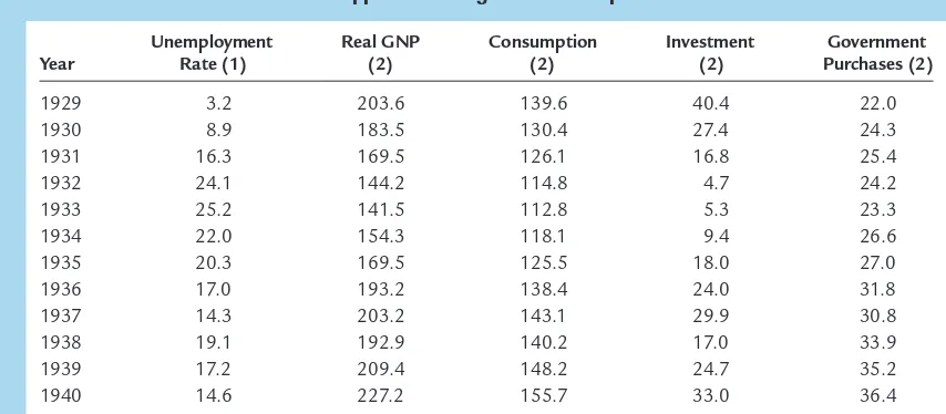
Before turning to the explanations economists have proposed, look at Table 11-2, which presents some statistics regarding the Depression.These statistics are the battlefield on which debate about the Depression takes place. What do you think happened? An ISshift? An LMshift? Or something else?
1For a flavor of the debate, see Milton Friedman and Anna J. Schwartz,A Monetary History of the
The Spending Hypothesis: Shocks to the
IS
Curve
Table 11-2 shows that the decline in income in the early 1930s coincided with falling interest rates. This fact has led some economists to suggest that the cause of the decline may have been a contractionary shift in the IScurve.This view is sometimes called the spending hypothesis,because it places primary blame for the Depression on an exogenous fall in spending on goods and services.
Economists have attempted to explain this decline in spending in several ways. Some argue that a downward shift in the consumption function caused the con-tractionary shift in the IScurve.The stock market crash of 1929 may have been partly responsible for this shift: by reducing wealth and increasing uncertainty about the future prospects of the U.S. economy, the crash may have induced con-sumers to save more of their income rather than spending it.
Others explain the decline in spending by pointing to the large drop in invest-ment in housing. Some economists believe that the residential investinvest-ment boom of the 1920s was excessive and that once this “overbuilding’’became apparent, the demand for residential investment declined drastically. Another possible ex-planation for the fall in residential investment is the reduction in immigration in the 1930s: a more slowly growing population demands less new housing.
Once the Depression began, several events occurred that could have reduced spending further. First, many banks failed in the early 1930s, in part because of inadequate bank regulation, and these bank failures may have exacerbated the fall in investment spending. Banks play the crucial role of getting the funds available
296| P A R T I V Business Cycle Theory: The Economy in the Short Run
Unemployment Real GNP Consumption Investment Government
Year Rate (1) (2) (2) (2) Purchases (2)
1929 3.2 203.6 139.6 40.4 22.0
1930 8.9 183.5 130.4 27.4 24.3
1931 16.3 169.5 126.1 16.8 25.4
1932 24.1 144.2 114.8 4.7 24.2
1933 25.2 141.5 112.8 5.3 23.3
1934 22.0 154.3 118.1 9.4 26.6
1935 20.3 169.5 125.5 18.0 27.0
1936 17.0 193.2 138.4 24.0 31.8
1937 14.3 203.2 143.1 29.9 30.8
1938 19.1 192.9 140.2 17.0 33.9
1939 17.2 209.4 148.2 24.7 35.2
1940 14.6 227.2 155.7 33.0 36.4
Source: Historical Statistics of the United States, Colonial Times to 1970, Parts I and II(Washington, DC: U.S. Department of Commerce, Bureau of Census, 1975).
Note:(1) The unemployment rate is series D9. (2) Real GNP, consumption, investment, and government purchases are series F3, F48, F52, and F66, and are measured in billions of 1958 dollars. (3) The interest rate is the prime Commercial
User JOEWA:Job EFF01427:6264_ch11:Pg 297:27344#/eps at 100%
*27344*
Wed, Feb 13, 2002 10:27 AM for investment to those households and firms that can best use them.The closingof many banks in the early 1930s may have prevented some businesses from get-ting the funds they needed for capital investment and, therefore, may have led to a further contractionary shift in the investment function.2
In addition, the fiscal policy of the 1930s caused a contractionary shift in the IS curve. Politicians at that time were more concerned with balancing the
bud-get than with using fiscal policy to keep production and employment at their natural rates. The Revenue Act of 1932 increased various taxes, especially those falling on lower- and middle-income consumers.3The Democratic platform of that year expressed concern about the budget deficit and advocated an “ immedi-ate and drastic reduction of governmental expenditures.’’In the midst of histori-cally high unemployment, policymakers searched for ways to raise taxes and reduce government spending.
There are, therefore, several ways to explain a contractionary shift in the IS curve. Keep in mind that these different views may all be true.There may be no single explanation for the decline in spending. It is possible that all of these changes coincided and that together they led to a massive reduction in spending.
Nominal Money Supply Price Level Inflation Real Money
Year Interest Rate (3) (4) (5) (6) Balances (7)
1929 5.9 26.6 50.6 − 52.6
1930 3.6 25.8 49.3 −2.6 52.3
1931 2.6 24.1 44.8 −10.1 54.5
1932 2.7 21.1 40.2 −9.3 52.5
1933 1.7 19.9 39.3 −2.2 50.7
1934 1.0 21.9 42.2 7.4 51.8
1935 0.8 25.9 42.6 0.9 60.8
1936 0.8 29.6 42.7 0.2 62.9
1937 0.9 30.9 44.5 4.2 69.5
1938 0.8 30.5 43.9 −1.3 69.5
1939 0.6 34.2 43.2 −1.6 79.1
1940 0.6 39.7 43.9 1.6 90.3
Paper rate, 4–6 months, series ×445. (4) The money supply is series ×414, currency plus demand deposits, measured in
billions of dollars. (5) The price level is the GNP deflator (1958 =100), series E1. (6) The inflation rate is the percentage change in the price level series. (7) Real money balances, calculated by dividing the money supply by the price level and multiplying by 100, are in billions of 1958 dollars.
2
Ben Bernanke,“Non-Monetary Effects of the Financial Crisis in the Propagation of the Great Depression,’’American Economic Review73 (June 1983): 257–276.
3
The Money Hypothesis: A Shock to the
LM
Curve
Table 11-2 shows that the money supply fell 25 percent from 1929 to 1933, dur-ing which time the unemployment rate rose from 3.2 percent to 25.2 percent. This fact provides the motivation and support for what is called the money hy-pothesis, which places primary blame for the Depression on the Federal Reserve for allowing the money supply to fall by such a large amount.4The best-known advocates of this interpretation are Milton Friedman and Anna Schwartz, who defend it in their treatise on U.S. monetary history. Friedman and Schwartz argue that contractions in the money supply have caused most economic down-turns and that the Great Depression is a particularly vivid example.
Using the IS–LM model, we might interpret the money hypothesis as ex-plaining the Depression by a contractionary shift in the LMcurve. Seen in this way, however, the money hypothesis runs into two problems.
The first problem is the behavior of real money balances. Monetary policy leads to a contractionary shift in the LMcurve only if real money balances fall. Yet from 1929 to 1931 real money balances rose slightly, because the fall in the money supply was accompanied by an even greater fall in the price level. Al-though the monetary contraction may be responsible for the rise in unemploy-ment from 1931 to 1933, when real money balances did fall, it cannot easily explain the initial downturn from 1929 to 1931.
The second problem for the money hypothesis is the behavior of interest rates. If a contractionary shift in the LM curve triggered the Depression, we should have observed higher interest rates.Yet nominal interest rates fell continu-ously from 1929 to 1933.
These two reasons appear sufficient to reject the view that the Depression was instigated by a contractionary shift in the LM curve. But was the fall in the money stock irrelevant? Next, we turn to another mechanism through which monetary policy might have been responsible for the severity of the Depres-sion—the deflation of the 1930s.
The Money Hypothesis Again: The Effects of
Falling Prices
From 1929 to 1933 the price level fell 25 percent. Many economists blame this deflation for the severity of the Great Depression.They argue that the deflation may have turned what in 1931 was a typical economic downturn into an un-precedented period of high unemployment and depressed income. If it is correct, this argument gives new life to the money hypothesis. Because the falling money supply was, plausibly, responsible for the falling price level, it could have been re-sponsible for the severity of the Depression.To evaluate this argument, we must discuss how changes in the price level affect income in the IS–LMmodel.
298| P A R T I V Business Cycle Theory: The Economy in the Short Run
4We discuss the reasons for this large decrease in the money supply in Chapter 18, where we
User JOEWA:Job EFF01427:6264_ch11:Pg 299:27346#/eps at 100%
*27346*
Wed, Feb 13, 2002 10:27 AMThe Stabilizing Effects of Deflation In the IS–LMmodel we have developed
so far, falling prices raise income. For any given supply of money M, a lower price
level implies higher real money balances M/P. An increase in real money balances
causes an expansionary shift in the LMcurve, which leads to higher income.
Another channel through which falling prices expand income is called the Pigou effect. Arthur Pigou, a prominent classical economist in the 1930s,
pointed out that real money balances are part of households’wealth. As prices fall
and real money balances rise, consumers should feel wealthier and spend more.
This increase in consumer spending should cause an expansionary shift in the IS
curve, also leading to higher income.
These two reasons led some economists in the 1930s to believe that falling prices would help stabilize the economy. That is, they thought that a decline in the price level would automatically push the economy back toward full
employ-ment.Yet other economists were less confident in the economy’s ability to
cor-rect itself. They pointed to other effects of falling prices, to which we now turn.
The Destabilizing Effects of Deflation Economists have proposed two theo-ries to explain how falling prices could depress income rather than raise it. The
first, called the debt-deflation theory, describes the effects of unexpected falls
in the price level.The second explains the effects of expected deflation.
The debt-deflation theory begins with an observation from Chapter 4:
unan-ticipated changes in the price level redistribute wealth between debtors and cred-itors. If a debtor owes a creditor $1,000, then the real amount of this debt is
$1,000/P, where Pis the price level.A fall in the price level raises the real amount
of this debt—the amount of purchasing power the debtor must repay the creditor.
Therefore, an unexpected deflation enriches creditors and impoverishes debtors.
The debt-deflation theory then posits that this redistribution of wealth affects
spending on goods and services. In response to the redistribution from debtors to creditors, debtors spend less and creditors spend more. If these two groups have equal spending propensities, there is no aggregate impact. But it seems reasonable
to assume that debtors have higher propensities to spend than creditors—perhaps
that is why the debtors are in debt in the first place. In this case, debtors reduce
their spending by more than creditors raise theirs.The net effect is a reduction in
spending, a contractionary shift in the IScurve, and lower national income.
To understand how expected changes in prices can affect income, we need to
add a new variable to the IS–LMmodel. Our discussion of the model so far has
not distinguished between the nominal and real interest rates.Yet we know from previous chapters that investment depends on the real interest rate and that
money demand depends on the nominal interest rate. If iis the nominal interest
rate and
p
eis expected inflation, then the ex antereal interest rate is i −p
e. Wecan now write the IS–LMmodel as
Y=C(Y−T) +I(i−
p
e) +G IS,M/P=L(i,Y) LM.
Expected inflation enters as a variable in the IScurve.Thus, changes in expected
Let’s use this extended IS–LM model to examine how changes in expected
inflation influence the level of income.We begin by assuming that everyone ex-pects the price level to remain the same. In this case, there is no expected infl a-tion (
p
e=0), and these two equations produce the familiar IS–LMmodel. Figure 11-8 depicts this initial situation with the LMcurve and the IScurve labeled IS1.The intersection of these two curves determines the nominal and real interest rates, which for now are the same.
Now suppose that everyone suddenly expects that the price level will fall in the future, so that
p
e becomes negative. The real interest rate is now higher at any given nominal interest rate.This increase in the real interest rate depresses planned investment spending, shifting the IScurve from IS1to IS2.Thus, an expectedde-flation leads to a reduction in national income from Y1to Y2.The nominal
inter-est rate falls from i1to i2, whereas the real interest rate rises from r1to r2.
Here is the story behind this figure. When firms come to expect deflation, they become reluctant to borrow to buy investment goods because they believe they will have to repay these loans later in more valuable dollars. The fall in in-vestment depresses planned expenditure, which in turn depresses income. The fall in income reduces the demand for money, and this reduces the nominal in-terest rate that equilibrates the money market.The nominal inin-terest rate falls by less than the expected deflation, so the real interest rate rises.
Note that there is a common thread in these two stories of destabilizing deflation. In both, falling prices depress national income by causing a contrac-tionary shift in the IS curve. Because a deflation of the size observed from
1929 to 1933 is unlikely except in the presence of a major contraction in the money supply, these two explanations give some of the responsibility for the Depression—especially its severity—to the Fed. In other words, if falling prices are destabilizing, then a contraction in the money supply can lead to a fall in income, even without a decrease in real money balances or a rise in nominal interest rates. Model An expected deflation (a
negative value of pe) raises the
real interest rate for any given nominal interest rate, and this depresses investment spending. The reduction in investment shifts
the IScurve downward. The level
of income falls from Y1to Y2. The
nominal interest rate falls from i1
to i2, and the real interest rate
User JOEWA:Job EFF01427:6264_ch11:Pg 301:27348#/eps at 100%
*27348*
Wed, Feb 13, 2002 10:27 AMCould the Depression Happen Again?
Economists study the Depression both because of its intrinsic interest as a major economic event and to provide guidance to policymakers so that it will not
hap-pen again. To state with confidence whether this event could recur, we would
need to know why it happened. Because there is not yet agreement on the causes of the Great Depression, it is impossible to rule out with certainty another de-pression of this magnitude.
Yet most economists believe that the mistakes that led to the Great Depression are unlikely to be repeated.The Fed seems unlikely to allow the money supply to
fall by one-fourth. Many economists believe that the deflation of the early 1930s
was responsible for the depth and length of the Depression. And it seems likely
that such a prolonged deflation was possible only in the presence of a falling
money supply.
The fiscal-policy mistakes of the Depression are also unlikely to be repeated.
Fiscal policy in the 1930s not only failed to help but actually further depressed aggregate demand. Few economists today would advocate such a rigid adherence to a balanced budget in the face of massive unemployment.
In addition, there are many institutions today that would help prevent the events of the 1930s from recurring. The system of Federal Deposit Insurance makes widespread bank failures less likely. The income tax causes an automatic reduction in taxes when income falls, which stabilizes the economy. Finally, economists know more today than they did in the 1930s. Our knowledge of how the economy works, limited as it still is, should help policymakers formulate better policies to combat such widespread unemployment.
C A S E S T U D Y
The Japanese Slump
During the 1990s, after many years of rapid growth and enviable prosperity, the Japanese economy experienced a prolonged downturn. Real GDP grew at an average rate of only 1.3 percent over the decade, compared with 4.3 percent over the previous twenty years.The unemployment rate, which had historically been very low in Japan, rose from 2.1 percent in 1990 to 4.7 percent in 1999. In Au-gust 2001, unemployment hit 5.0 percent, the highest rate since the government began compiling the statistic in 1953.
Although the Japanese slump of the 1990s is not even close in magnitude to the Great Depression of the 1930s, the episodes are similar in several ways. First, both episodes are traced in part to a large decline in stock prices. In Japan, stock prices at the end of the 1990s were less than half the peak level they had reached about a decade earlier. Like the stock market, Japanese land prices had also skyrocketed in
the 1980s before crashing in the 1990s. (At the peak of Japan’s land bubble, it was
11-4
Conclusion
The purpose of this chapter and the previous one has been to deepen our under-standing of aggregate demand. We now have the tools to analyze the effects of
monetary and fiscal policy in the long run and in the short run. In the long run,
prices are flexible, and we use the classical analysis of Parts II and III of this book.
In the short run, prices are sticky, and we use the IS–LMmodel to examine how
changes in policy influence the economy.
302| P A R T I V Business Cycle Theory: The Economy in the Short Run
Second, during both episodes, banks ran into trouble and exacerbated the slump in economic activity. Japanese banks in the 1980s had made many loans that were backed by stock or land. When the value of this collateral fell, bor-rowers started defaulting on their loans. These defaults on the old loans
re-duced the banks’ ability to make new loans. The resulting “credit crunch”
made it harder for firms to finance investment projects and, thus, depressed in-vestment spending.
Third, both episodes saw a fall in economic activity coincide with very low interest rates. In Japan in the 1990s, as in the United States in the 1930s, short-term nominal interest rates were less than 1 percent. This fact suggests that the
cause of the slump was primarily a contractionary shift in the IScurve, because
such a shift reduces both income and the interest rate. The obvious suspects to
explain the ISshift are the crashes in stock and land prices and the problems in
the banking system.
Finally, the policy debate in Japan mirrored the debate over the Great Depres-sion. Some economists recommended that the Japanese government pass large tax cuts to encourage more consumer spending. Although this advice was fol-lowed to some extent, Japanese policymakers were reluctant to enact very large tax cuts because, like the U.S. policymakers in the 1930s, they wanted to avoid
budget deficits. In Japan, this reluctance to increase government debt arose in
part because the government was facing a large unfunded pension liability and a rapidly aging population.
Other economists recommended that the Bank of Japan expand the money supply more rapidly. Even if nominal interest rates could not go much lower, then perhaps more rapid money growth could raise expected inflation, lower real interest rates, and stimulate investment spending. Thus, although econo-mists differed about whether fiscal or monetary policy was more likely to be
effective, there was wide agreement that the solution to Japan’s slump, like the
solution to the Great Depression, rested in more aggressive expansion of
ag-gregate demand.5