Price and inventory dynamics in petroleum
product markets
Timothy J. Considine
a,U, Eunnyeong Heo
b aDepartment of Energy, En¨ironmental, and Mineral Economics, The Pennsyl¨ania State Uni¨ersity, 203 Eric A. Walker Building, Uni¨ersity Park, PA 16802, USA
b
School of Ci¨il, Urban, and Geosystem Engineering, Seoul National Uni¨ersity, San 56-1, Shinrim, Kwanak, Seoul 151-742, South Korea
Abstract
Unlike many studies of commodity inventory behavior, this paper estimates a model with endogenous spot and forward prices, inventories, production, and net imports. Our applica-tion involves markets for refined petroleum products in the United States. Our model is built around the supply and demand for storage. We estimate the model using Generalized Method of Moments and perform dynamic, simultaneous simulations to estimate the impacts of supply and demand shocks. Supply curves for the industry are inelastic and upward sloping. High inventory levels depress prices. Inventories fall in response to higher sales, consistent with production smoothing. Under higher input prices, refiners reduce their stocks of crude oil but increase their product inventories, consistent with cost smoothing. In some cases, imports of products are more variable than production or inventories.䊚 2000 Elsevier Science B.V. All rights reserved.
JEL classifications:C5; L6; Q4
Keywords:Inventories; Convenience yield; Petroleum
1. Introduction
The second half of the 1980s was a period of rapid change in US petroleum markets. The introduction of a netback pricing system by Saudi Arabia in late 1985, followed by the crude oil price collapse in 1986, ushered in a flexible pricing system
UCorresponding author. Tel.:q1-814-863-0810; fax:q1-814-863-7433.
Ž . Ž .
E-mail addresses:[email protected] T.J. Considine , [email protected] E. Heo . 0140-9883r00r$ - see front matter䊚2000 Elsevier Science B.V. All rights reserved.
Ž .
with spot and futures markets. Crude oil and petroleum product markets now have become fully developed through the 1990s. As these new markets matured, changes within them became an important part of the decision-making process of the US petroleum refining industry. Market prices of petroleum products now appear quite sensitive to supply and demand shocks, unlike the previous era of pricing under long-term contracts.
As a result, inventories now play an important role in the transmission of these market shocks to petroleum product prices. Petroleum inventories are assets, and their valuation by refiners varies with market conditions. For example, as futures or forward prices rise above spot or cash prices, the user cost of inventories decline, and refiners may increase stock holding to reap expected profits at some point in the future. Similarly, relatively higher spot prices raise incentives to lower invento-ries, which may reduce pressure on prices for current delivery. Hence, inventories affect the adjustment of the petroleum markets to OPEC production decisions, weather, and other market shocks.
Understanding the linkages between prices, inventories, and production in the petroleum refining industry is our objective. We expand on the studies of these
Ž .
interactions by Bacon et al. 1980 using a model suitable for econometric estima-tion and simulaestima-tion. We estimate the model using monthly data from 1985 to 1996, conduct a goodness-of-fit simulation, and perform a set of simulations to under-stand how petroleum markets respond to market shocks.
We model short-run petroleum price and inventory movements using a sequence of submodels. In the first model, we assume petroleum refiners minimize cost given exogenous output targets and prices for inputs. We consider inventories as a quasi-fixed factor of production with rental costs that include expected prices for petroleum products. The second model determines spot and nearby futures prices also contingent upon production, sales, and input prices. In this component, we formulate the model viewing prices as a stochastic state variable.
Why do we adopt this approach? The rational expectations models of commodity
Ž . Ž .
price and inventory dynamics developed by Pindyck 1994 and Considine 1997 contain equilibrium conditions for inventories that essentially equate the marginal costs and benefits of inventories, including a convenience yield earned from the cost and production smoothing benefits from holding inventories. These dynamic demand functions for inventories, however, are overidentified, containing expecta-tions of future inventories, production, and prices. While this formulation facili-tates econometric estimation, it greatly complicates model simulation because solutions for expectations are required. In contrast, this paper provides an explicit, closed form model for price expectations. Our approach is driven by the desire to have a model motivated by theory yet flexible enough to allow dynamic simulation for forecasting and policy analysis.
assume total domestic sales of petroleum products are exogenous and solve for production by adding net inventory changes and net exports to domestic consump-tion. Overall, our model determines prices, inventories, production, net imports for petroleum products in the US contingent upon exogenously determined product consumption, crude oil prices, and prices for other factor inputs.
We assume refiners are price takers in crude oil and in petroleum product
Ž .
markets. A multiproduct formulation along the lines of Griffin 1976 is also adopted in this study to reflect joint production in petroleum refining. Crude oil and petroleum liquids are the two variable inputs in the model, constituting roughly 95% of the variable cost of petroleum refining. To reduce the size and complexity of the model, we examine five product aggregatesᎏ gasoline, distillate fuel, residual fuel, jet fuel, and other petroleum products, and only the first four products are considered for the price᎐arbitrage relations due to the unavailability of data on prices for other petroleum products.
Section 2 contains the theoretical foundations of the empirical model. The functional specification of the econometric equations appears in Section 3, fol-lowed by a summary of the estimation results in Section 4. The last section contains simulations to test the model’s forecasting ability and to estimate the market impacts of supply and demand shocks.
2. Model formulation
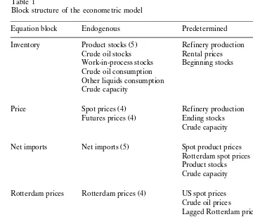
The primary objective of this study is to develop a structural model of refined petroleum product markets suitable for simulation and forecasting. To provide an overview of the model, we devised the following block structure, summarized in Table 1. There are five major blocks in the model that determine groups of endogenous variables contingent upon predetermined and exogenous variables. The latter are determined outside the entire model whereas predetermined vari-ables depend upon some other block. The exogenous varivari-ables include crude oil and propane prices, weather conditions measured by heating and cooling degree-days, interest rates, petroleum product sales, and storage costs.
Table 1
Block structure of the econometric model
Equation block Endogenous Predetermined Exogenous
Ž .
Inventory Product stocks 5 Refinery production Crude prices
Crude oil stocks Rental prices Propane prices
Work-in-process stocks Beginning stocks Weather
Crude oil consumption Interest rates
Other liquids consumption Crude capacity
Ž .
Price Spot prices 4 Refinery production Crude prices
Ž .
Futures prices 4 Ending stocks Propane prices
Crude capacity
Ž .
Net imports Net imports 5 Spot product prices Product sales
Rotterdam spot prices Weather Product stocks
Crude capacity
Ž .
Rotterdam prices Rotterdam prices 4 US spot prices Crude prices Crude oil prices
Rental prices Rental prices 8 Spot prices Storage costs
Futures prices Interest rates Crude prices Propane prices
predictions of spot and futures prices from the price block and refinery production given inventories and net imports from the first and third blocks, respectively.
We formulate the inventory block using a dynamic dual formulation. Many researchers have exploited the duality between cost and production functions to derive input demand functions consistent with either cost minimization or profit
Ž . Ž .
maximization. Following the earlier work by Lucas 1967 and Treadway 1971 on
Ž .
the flexible accelerator model, McLaren and Cooper 1980 and Epstein and
Ž .
Denny 1983 have extended the dual approach to dynamic problems.
A dynamic problem often embodies the distinction between the short run when some factors of production are fixed and the long run when all factors can adjust to equilibrium levels. Adjustment costs are often claimed as the reason for dichotomy. These costs are generally unobservable and are often expressed as the reduction in output resulting from diverting resources to accommodate changes in quasi-fixed factors of production.
capacity levels. In addition, adjusting inventories may be costly due to logistical differences in transport and scheduling. Consequently, we consider the following short-run restricted cost function for a petroleum product firm:
Ž . Ž .
G w,y,x,
˙
x sminimize wz, 1where G is the variable cost function; w is a vector of prices for crude oil and propane; y the vector of refinery production levels; x the vector of quasi-fixed factors;
˙
x the vector of changes in levels of quasi-fixed factors; and z the vector of variable inputs.The vector of variable inputs z is the choice variable in the cost minimization problem and is subject to a production function:
Ž . Ž .
F y,z,x,
˙
x s0 . 2Note that Fx)0, Fz)0 and Fx˙-0, in which the last derivative reflects internal adjustment costs.
Assume that the firm attempts to minimize the present discounted value of future costs over an infinite horizon at some point in time ᎏ say period ts0, by adjusting variable input purchases and net accumulations of quasi-fixed factors. In this case, given initial states for the quasi-fixed factors, x0, exogenous prices for variable and quasi-fixed inputs, and predetermined levels of output, the discounted value function J is:
⬁ yr t
Ž . w Ž . x Ž .
J x0,y,w,¨ smin
H
e G w,y,x,˙
x q¨⬘x dt, 30
subject to positive starting values for the quasi-fixed factors, and where ¨ is the vector of rental costs for quasi-fixed factors and r is a fixed discount factor.
The discounted value function is assumed to be real, non-negative, twice contin-uously differentiable, non-decreasing, and concave inw and¨ and decreasing in x
ŽEpstein and Denny, 1983 . Under these conditions, the Hamilton. ᎐Jacobi᎐Bellman
Ž .
expression Kamien and Schwartz, 1991 ᎏ often referred to as the dynamic programming equation, is as follows:
⬁ yr t
Ž . w Ž . x Ž .
J x0,y,w,¨ smin
H
e G w,y,x,˙
x q¨⬘xq˙
x⬘Jx dt. 4 0This equation simply states that the discounted long-run cost is equal to the sum of total variable costs, total rental costs of the quasi-fixed factors¨⬘x, and the implicit
Ž .
value of additional fixed factors
˙
x⬘Jx Stefanou, 1989 .With this restatement of the objective function, we derive a set of first-order conditions for the dynamic problem. Consider one such condition involving the rate of change in quasi-fixed factors
˙
x:Ž .
which states that the marginal adjustment costs of the quasi-fixed factors in any period must equal their respective shadow values. Also, consider the first-order condition with respect to the level of quasi-fixed factors x:
Ž . Ž .
¨⬘s y GxqJ xx x
˙
, 6which implies that rental values should reflect the shadow value and net capital
Ž .
gains from stock holding. If we differentiate Eq. 4 with respect to ¨, we obtain:
⭸
˙
xU ⭸xUU Ž . Ž . Ž .
rJ¨sxqx J
˙
x¨q G˙xqJx ⭸¨ q ¨⬘qGxqJx x ⭸¨ , 7Ž . Ž .
where the asterisks indicate evaluation at optimal values. Using Eqs. 5 and 6
Ž . U
and solving Eq. 7 for x
˙
, we obtain the following expression for optimal net investment in quasi-fixed factors:The demand for the variable input can be obtained by differentiating Eq. 4 with
Ž U .
respect to w and using Shephard’s lemma z s⭸Gr⭸w to obtain:
U Ž .
z srJwy
˙
x⬘Jx w. 9The above problem involves the optimal choice of variable and quasi-fixed factors
Ž . Ž .
to minimize cost. Eq. 8 determines the demand for storage while Eq. 9 consti-tutes the demand for variable inputs.
To determine equilibrium spot and futures prices, we develop a model of the
Ž .
supply for storage. As Brennan 1958 notes, this supply is not the supply of storage space but the supply of commodities as inventories. A supplier of storage is anyone who holds title to stocks for future sale, including hedgers and speculators. We will collectively call these agents oil traders. We assume that price is a stochastic state
Ž .
variable analogous to the study by Considine and Larson 1998 and that traders choose sales and production to maximize their expected present value of profits:
⬁ yr t
where db is the standard Weiner process,1 s is total domestic sales, dx is ending
1A Weiner process has three important properties. First, it is a Markov process so that the current
Ž .
less beginning inventories, and n is imports less exports, C x,y,w,k,h represents the cost of production, marketing, and transportation of refined petroleum products,
2
Ž .
k is capacity, and h represents technological change. Eq. 11 simply rewrites the market balance equation, which states that sales must come from current
produc-w tion, net imports, and the net change in stocks. We assume the price process Eq.
Ž12.xevolves stochastically over time, following geometric Brownian motion with a
Ž . Ž .
drift component, p, and a variance, p. This assumption allows us to derive an expression for the supply of storage. This derivation begins with the Bellman equation for this problem:
The partial differentials with respect to sales and production imply the following first-order conditions:
rVsspyVxs0«psVx
Ž .
, 14
rVys yCyqVxs0«psCy
indicating that equilibrium prices reflect marginal production costs and the shadow value of inventories. An expression for the expected change in prices follows from
Ž .
differentiating Eq. 14 using Ito’s lemma:
Ž .
Differentiating Eq. 13 with respect to x and solving for Cx provides the convenience yield:
which equals the expected capital gain on inventories Eq. 15 net of interest costs. Notice that for the convenience yield to reflect the variability in prices, the value function must have non-zero third-order derivatives.
2
The introduction of a cost function for traders separates the inventory block from the price block.
Ž .
Considine 1992 derives a supply function from the dual profit maximization problem associated with
Ž .
Ž . Ž . Ž .
Substituting Eqs. 14 and 16 into Eq. 15 , we obtain the supply of storage relation, which is a simple relation for the expected change in prices:
Ž .
E dp
Ž .
sCxyrp. 17
dt
This relation states that the expected capital gain reflects the convenience yield net
Ž .
of interest costs. During so-called market backwardations when Edp is negative, Cx could be large and negative, indicating that another barrel of inventory could
Ž . Ž .
substantially lower costs or provide a high con¨enience yield. Eqs. 14 and 17 constitute the basis of an empirical model once we specify a cost function and its derivatives. Estimation of the supply of storage model also could be accomplished with an approximation of the value function. We adopt the cost function approach
Ž .
because it does not require estimation of Eq. 15 .
w Ž .x
The demand for storage Eq. 8 is contingent upon a sequence of production targets. In other words, vertically integrated petroleum refining firms minimize cost
w Ž .x
subject to production levels. The supply of storage Eq. 17 relation defines an equilibrium relation between expected prices and inventories. Together these relations determine the supply and demand for inventories and the equilibrium
Ž .
price for storage given by Eq. 17 .
If sales are given in the short-run by weather, income, and other exogenous factors, then production is simply sales plus the net inventory change less net imports. This implies that with a model of net foreign trade of petroleum products, we can solve for production using the market balance equation:
Ž .
yssqdxyn . 18
Conditional upon market prices, we assume traders minimize their net import product expenditures for each product subject to capacity, ending stocks, and final product shipments. We assume these decisions are strongly separable from inven-tory and production decisions to simplify the model. With the assumption that both imports and exports sell at the same price, we obtain the demand for net imports by the first-order condition of this problem with respect to the import price, using Shephard’s lemma:
where NE is the net import expenditure function, and pr is a vector of prices for imported petroleum products.
3. Empirical model
Ž
dual models utilize a second-order linear quadratic approximation Epstein and
.
Denny, 1983; Stefanou et al., 1992 . Another approach is to use translog or
Ž .
generalized Leontief approximations as in Luh and Stefanou 1996 . Such forms, however, must be modified to accommodate the linear adjustment mechanism in
w Ž .x
the optimal net investment equation of quasi-fixed factors Eq. 8 . As a result, this study uses a quadratic approximation of the value function for the inventory and demand module to avoid potential convergence problems with these mixed func-tional forms.
A normalized quadratic formulation is typically used for the approximation so that linear homogeneity in prices can be imposed on the cost function. However,
Ž .
Mahmud et al. 1986 finds that parameter estimates from normalized models vary depending upon the selection of the normalizing numerator. Therefore, this study utilizes an unrestricted model that is not homogeneous in factor prices. Following
Ž .
Miron and Zeldes 1988 , heating and cooling degree-day deviations are included in the cost function to random weather shocks. The quadratic value function for the inventory and demand module then takes the following form:
w
where the variables are defined as follows:
䢇 w is a 2=1 vector of real prices for the refiners’ acquisition cost of crude oil and propane;
䢇 y is a 5=1 vector of refinery production of gasoline, distillate, residual fuel, jet fuel and kerosene, and other petroleum products;
䢇 x is an 8=1 vector of seven inventory categories, including crude oil and liquids, unfinished oils, the five products, and crude distillation capacity;
Ž .
䢇 ¨ is an 8=1 vector of rental values or user costs for the quasi-fixed factors; and
The e vectors are random error terms that reflect errors in dynamic
optimiza-Ž .
tion. The other terms on the right-hand side of Eq. 20 are unknown parameters to be estimated.
The estimating equations for the net investment in quasi-fixed factors follow from taking the derivative of value function J with respect to ¨, x, and u and
Ž .
substituting into Eq. 8 :
U Ž . Ž . Ž .
x srM a qg⬘wqB¨ qHyqf u q rIyM xqrMe . 21
˙
¨ ¨ ¨ ¨Note that if the error terms are serially correlated, they must move at the rate of adjustment M.
Ž .
The study by Epstein and Denny 1983 transforms the non-linear structural
Ž .
form given by Eq. 21 into a linear reduced-form model. To derive the reduced
Ž .
form for estimation, we express Eq. 21 as follows:
U Ž . Ž . Ž .
Substituting Eq. 23 into Eq. 22 using the discrete approximation xyxy1 for
U Ž . Ž .
x and xy1yx for xyx , we obtain the following partial adjustment equations for the quasi-fixed factors:
w x wŽ . x Ž .
xsrM a¨qg⬘¨wqB¨ qHyqf u¨ q 1qr IyM xy1qrMe¨. 24
Ž .
The terms in the first set of brackets on the right-hand side of Eq. 24 constitute the target or long-run equilibrium level of stocks. These targets depend upon crude oil cost shocks, rental values, final product sales, and weather shocks represented by u.Given that the adjustment coefficients M are identified, we can estimate the
Ž
model in reduced form and recover the structural parameters Epstein and Denny,
.
1983 .
The demands for the variable inputs are obtained by taking the derivative of J
Ž .
and Jx and with respect to w and substituting into Eq. 9 :
Ž . Ž . Ž .
zsr awqg⬘wwqg¨¨ qg xx qg yy qf uw yg xx yxy1 qrew. 25
Ž .
The second to last term on the right of Eq. 25 represents the extent of
Ž . Ž .
h11 h12 h13 h14 h15 h21 h22 h23 h24 h25
h31 0 0 0 0
0 h42 0 0 0
Ž .
Hs . 26
0 0 h53 0 0
0 0 0 h64 0
0 0 0 0 h75
h81 h82 h83 h84 h85
Thus, refinery production levels for all products affect refinery capacity, crude oil, and work-in-process inventories, while product inventories only depend on their own production level.
Given these assumptions, the estimating equations for the refinery inventory and demand module are as follows:
2 5
) ) ) )
xi tsr a¨iq
Ý
g w¨i j jtqbi i¨ qi tÝ
h yi j jtqf ui h h tqf ui c c tjs1 js1
Ž . ) Ž .
q 1qrymi i xi ty1qei t , 27
for is1, 2, 8, which are the demand for crude oil and unfinished inventories, and crude distillation capacity;
2
) ) ) )
xi tsr a¨iq
Ý
g w¨i j jtqbi i¨ qi t hi iy2yiy2tqf ui h h tqf ui c c t js1Ž . ) Ž .
q 1qrymi i xi ty1qei t , 28
for is3, . . . ,7, which constitute the demands for product storage; and
2 8 5
zi tsr aw iq
Ý
g w¨i j jtqÝ
gx i j jtx qÝ
gy i j jty qfz i huh tqfz i cuc tjs1 js1 js1
8
)
Ž . Ž .
y
Ý
gx i j xjtyxjty1 qew t, 29 js1for is1, 2, which are the equations for consumption of crude oil and propane. Note that the investment equations are in reduced form, so that hUi jsm hi i i j. All the quasi-fixed factors, x, depend on input prices w,own-user cost ¨, production levels y, weather u, and an own-lag term weighted by the adjustment coefficients m. The demands for variable inputs are unaffected by user costs for quasi-fixed factors but change with quasi-fixed factors. They also depend on the input prices, production levels for all products, and weather.
requires that its corresponding value and cost functions have at least non-zero third᎐order derivatives. To conform to the non-zero third-order derivative require-ment, we assume a square-root quadratic approximation for the trader’s cost
Ž .
function. Using Eq. 14 , we estimate the following expression for spot prices for refinery products: ␦i js␦ji given symmetry. In other words, spot prices depend upon input prices, production, own product inventory, capacity, and a time trend for technological change.
Ž .
Using Eq. 17 , the returns-to-storage equation is as follows, using the difference between the 1-month futures price and the spot price for the expected price change:
for is1,...,4, where pfi t is the nearby futures price. In the model simulations reported below, we solve this expression for the futures prices. The spot price and the arbitrage relations for the refinery products, are affected by input prices, inventory and production levels of all products, capacity k, and time trend t. In addition, the arbitrage relations depend on the opportunity cost of capital. As in
Ž . Ž .
Considine and Larson 1998 and Heo 1998 , this study also hypothesizes that futures and spot prices affect current inventory levels.
The estimated form of the net import equations are obtained by applying Eq.
Ž19 to a simple quadratic function for the net import expenditure function for.
each product:
Ž .
ni tsaeiqhi i pri tr pi t qki,iq2xiq2 ,tqk xi8 8tql si i i tqr ui h h tqr ui c c tqei t,
Ž32.
for is1, . . . ,5. This formulation essentially implies strong separability between various net product import demands. One-time lags of independent variables are added to each estimation equation to treat autocorrelation.
facilitate this model’s forecasting ability. This study adopts four simple autoregres-sive models for Rotterdam product spot prices for the import price module, which
Ž .
were originally proposed by the Energy Information Administration 1993 :
Ž .
pri tsspriqsp pi i tqsc wi tqsl pri i,ty1, 33
for is1, . . . ,4, where pr, p andw are the vectors of Rotterdam spot prices, New York spot prices, and crude oil price, respectively.
User costs for inventories are defined as the sum of the financial opportunity cost of capital, storage cost and the difference between futures and spot prices:
f
Ž .
¨ si t rpi tqsty pi typi t , 34
for is1,...,7. Again, for model simulation, estimates of spot prices provided by Eq.
Ž30 and futures prices given by Eq. 31 would make user costs an endogenous. Ž .
variable in the model. A similar rental price formulation is used for crude distillation capacity, except storage costs are replaced by depreciation.
The entire refined petroleum market model consists of 27 behavioral equations:
w Ž . Ž .x
䢇 the seven inventory and the capacity equations Eqs. 27 and 28 , and the two
w Ž .x
variable input demand functions Eq. 29 for the refinery inventory and demand module;
w Ž .x w
䢇 the four spot price equations Eq. 30 and the four arbitrage relations Eq.
Ž31 ;.x
w Ž .x
䢇 the five net product import equations Eq. 32 for the net import module; and
w Ž .x
䢇 the four imported oil price equations Eq. 33 for the import price module.
Ž .
In addition, there are the market clearing identities defined in Eq. 18 and the
Ž .
user cost definitions given by Eq. 34 .
4. Empirical analysis
We estimate each of the four modules separately to avoid convergence problems that may occur when estimating large simultaneous equation systems. Our
estima-Ž . Ž .3
tor is the Generalized Method of Moments GMM developed by Hansen 1982 . The lags on the moving average components of the errors are from the optimal
Ž .
bandwidths formulas developed by Newey and West 1994 . All variables in the
Ž .
model are stationary. Using the methods developed by Hylleberg et al. 1990 , we also found no seasonal unit roots.
The instrumental variables used in this study are seasonally unadjusted. They include the M1 measure of the money supply, housing starts, manufacturing labor hours, consumer price index net of energy, the S & P 500 index, the industrial
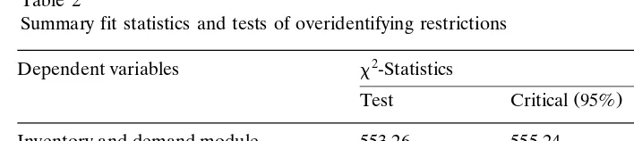
Table 2
Summary fit statistics and tests of overidentifying restrictions
2
Dependent variables -Statistics
Ž .
Test Critical 95% P-Value
Inventory and demand module 553.26 555.24 0.06
Price module 439.35 519.44 0.82
Net import module 319.65 320.03 0.05
Import price module 260.75 298.61 0.48
production index, long-term bond rates, yields on federal funds, and deviations of heating and cooling degree days from their 30-year means. Lagged values of refinery productions, net imports, NYMEX and Rotterdam spot prices, inventories of petroleum products, and lagged world petroleum production are also included. In addition, four OPEC regime shift variables are included for the crude oil price collapse from February to November 1986, the invasion of Kuwait by Iraq on August 1990, and the ‘Desert Shield’ and ‘Desert Storm’ from September to December 1990 and from January to February 1991, respectively. A set of monthly dummy variables is also included to account for fixed seasonal effects.
Estimation uses monthly data from January 1985 to December 1994. The input price vector includes propane prices and the refiner acquisition price for crude oil, which includes domestic and imported supplies. We use spot and 1-month futures prices for gasoline and heating fuel from the New York Mercantile Exchange
ŽNYMEX for current and expected prices. Import product prices are Rotterdam.
spot prices. Jet fuel prices equal an average of gasoline, distillate, and residual prices and residual fuel futures prices equal crude oil futures for prices due to data unavailability. Inventories are month-end values. Consequently, we used month-end prices for crude oil and products. All other data are monthly averages from the
Ž .
Department of Energy’s Energy Information Administration EIA database. We found that the model was much more stable in out-of-sample simulations when we included monthly dummies in the input and product inventory equations. Thus, the inventory equations contain fixed seasonal effects captured by the monthly dummy variables and stochastic weather effects represented by deviations of heating and cooling degree-days from their 30-year means.
First, we performed tests for the overidentifying restrictions of the model to test the maintained restrictions, such as dynamic optimization, and the quadratic approximation of the cost function.4 The P values of the test are larger than 0.05
Ž .
for all modules, indicating that we cannot reject the four modules see Table 2 . The estimated residuals have no unit root at the 5% significance level in aug-mented Dickey᎐Fuller tests, indicating an absence of serious dynamic misspecifica-tion.
Values of the estimated parameters are listed in Table A1 through Table A4 of
4
Ž .
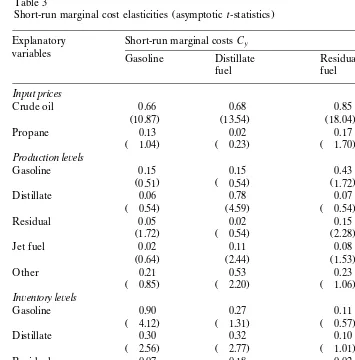
Table 3
Ž .
Short-run marginal cost elasticities asymptotict-statistics Explanatory Short-run marginal costsCy
variables Gasoline Distillate Residual Jet
fuel fuel fuel
Input prices
Crude oil 0.66 0.68 0.85 0.72
Ž10.87. Ž13.54. Ž18.04. Ž15.03.
Propane y0.13 y0.02 y0.17 y0.08
Žy1.04. Žy0.23. Žy1.70. Žy0.83.
Production le¨els
Gasoline 0.15 y0.15 0.43 0.13
Ž0.51. Žy0.54. Ž1.72. Ž0.64.
Distillate y0.06 0.78 y0.07 0.24
Žy0.54. Ž4.59. Žy0.54. Ž2.44.
Residual 0.05 y0.02 0.15 0.04
Ž1.72. Žy0.54. Ž2.28. Ž1.53.
Jet fuel 0.02 0.11 0.08 0.08
Ž0.64. Ž2.44. Ž1.53. Ž2.05.
Other y0.21 y0.53 y0.23 y0.32
Žy0.85. Žy2.20. Žy1.06. Žy1.58.
In¨entory le¨els
Gasoline y0.90 y0.27 y0.11 y0.45
Žy4.12. Žy1.31. Žy0.57. Žy2.60.
Distillate y0.30 y0.32 y0.10 y0.26
Žy2.56. Žy2.77. Žy1.01. Žy2.62.
Residual y0.07 0.18 y0.02 0.02
Žy1.17. Ž2.37. Žy0.24. Ž0.41.
Jet fuel y0.13 y0.01 y0.01 y0.02
Žy4.18. Žy0.27. Žy0.21. Žy0.55.
Other 0.04 0.17 0.16 0.13
Ž0.20. Ž0.83. Ž0.91. Ž0.76.
Capacity 0.80 y0.64 y1.07 y0.32
Ž2.01. Žy1.62. Žy2.99. Žy0.96.
Time 0.08 0.08 0.12 0.10
Ž1.11. Ž1.19. Ž2.00. Ž1.64.
Appendix A. Among the seven user cost terms in the inventory equations, those of gasoline, distillate, jet fuel, and other petroleum products stocks are negative, showing correct signs consistent with the theory of storage. Estimated rates of adjustment mi i for inventories are rapid. For gasoline, 29% of the total adjustment of stocks occurs within 1 month. The adjustment rate for residual fuel is even quicker with more than half of the adjustment occurring within 1 month. These rates suggest that, on average, it may take less than 6 months for the petroleum stocks to adjust to equilibrium levels.
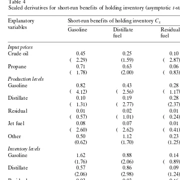
Table 4
Ž .
Scaled derivatives for short-run benefits of holding inventory asymptotict-statistics Explanatory Short-run benefits of holding inventoryCx
variables Gasoline Distillate Residual Jet
fuel fuel fuel
Input prices
Crude oil y0.45 0.25 y0.10 y0.09
Žy2.29. Ž1.59. Žy2.87. Žy1.02.
Propane y0.71 0.63 y0.06 y0.06
Žy1.78. Ž2.00. Žy0.83. Žy0.35.
Production le¨els
Gasoline y0.82 y0.43 y0.28 y0.47
Žy4.12. Žy2.56. Žy1.17. Žy4.18.
Distillate y0.10 y0.19 0.28 y0.01
Žy1.31. Žy2.77. Ž2.37. Žy0.27.
Residual y0.01 y0.02 y0.01 0.00
Žy0.57. Žy1.01. Žy0.24. Žy0.21.
Jet fuel y0.08 y0.07 y0.01 y0.01
Žy2.60. Žy2.62. Žy0.41. Žy0.55.
Other 0.50 1.12 0.23 0.62
Ž0.62. Ž1.70. Ž1.25. Ž1.99.
In¨entory le¨els
Gasoline 1.62 0.88 y0.14 0.77
Ž1.76. Ž2.06. Žy0.89. Ž2.46.
Distillate 0.57 0.86 0.09 0.51
Ž2.06. Ž2.98. Ž1.24. Ž4.29.
Residual y0.03 0.03 0.16 0.03
Žy0.89. Ž1.24. Ž1.44. Ž0.61.
Jet fuel 0.19 0.19 0.03 0.14
Ž2.46. Ž4.29. Ž0.61. Ž3.36.
Other y0.74 0.91 y0.29 y0.04
Žy1.10. Ž1.56. Žy2.05. Žy0.16.
Capacity y0.08 y4.31 0.23 y1.41
Ž0.06. Žy4.81. Žy0.78. Žy2.50.
Time 0.15 0.14 y0.15 y0.03
Ž0.70. Ž0.84. Žy3.37. Žy0.37.
preparation for higher gasoline demand as summer approaches. Inventories and variable input demands all rise with higher production.
In the price module, spot prices increase with higher crude oil prices and
Ž .
own-production levels see Table 3 . All four short-run price equations conform to the conventional notion of an upward sloping supply curve. In addition, several of the cross-elasticities of marginal cost with respect to production are significant, indicating joint production interactions. Spot prices also decline with higher ‘own’ inventory levels ᎏ significantly for gasoline and distillate fuels.
level of the variable in the partial equilibrium differentiation. The scaled deriva-tives of the estimatedCx function with respect to own inventory levels are positive and significant, consistent with the theory of storage. Negative scaled derivatives
Ž .
with respect to own-production levels indicate that theCx functions shift up down
Ž .
with lower higher production levels. This finding suggests that, ceteris paribus, marginal convenience yields increase when production declines.
Ratios of Rotterdam and NYMEX spot prices play a limited role in net imports. Own-product shipment levels have positive effects on most net imports, indicating that refiners import more as product demands increase. Capacity and weather variables have very little effect on petroleum product net imports. The import price equations show significant positive correlation between Rotterdam and NYMEX spot prices.
5. Simulation analysis
The simulation model consists of 41 equations, which we solve simultaneously. In addition to the 27 behavioral equations, we include five refinery product produc-tion identities based on the material balances for out-of-sample forecasting. The simulation model also includes an identity for gross product worth, which is a weighted average of product prices, and seven identities that define user costs for quasi-fixed factors. Finally, the model includes an equation for net refinery processing gains by simply taking the difference between total refining inputs and outputs.
Ž .
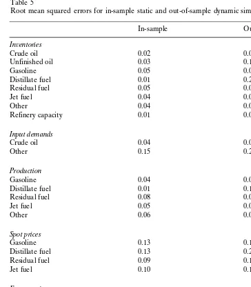
We first performed a static simulation of the model see Table 5 . Inventories
Ž .
and production forecasts show very low root mean squared errors RMSEs , less than 5% on average. RMSEs of the product spot and futures prices are relatively higher than those of inventory equations averaging slightly higher than 10%. The model shows very good fits for refinery production and inventories; all with lower than 10% RMSEs, except for those of distillate fuel. Finally, the model does not display any explosive tendencies during all simulations even with different sets of prices5, further illustrating the model’s stability. These goodness-of-fit simulations imply that the model would perform well in evaluating future policy implications. The next test of the model involves measuring the impacts associated with demand and supply shocks. Our demand shock involves a colder than average winter over a 3-month period represented by a 10% increase in heating degree-days. The model assumes final product sales are exogenous. To estimate the impacts of weather on product sales, we estimate five simple product demand equations that
5Month-average prices, such as average spot prices and resale prices, when compared to the results
Table 5
Root mean squared errors for in-sample static and out-of-sample dynamic simulation solutions
In-sample Out-of-sample
In¨entories
Crude oil 0.02 0.09
Unfinished oil 0.03 0.10
Gasoline 0.05 0.09
Distillate fuel 0.01 0.21
Residual fuel 0.05 0.09
Jet fuel 0.04 0.06
Other 0.04 0.09
Refinery capacity 0.01 0.01
Input demands
Crude oil 0.04 0.04
Other 0.15 0.25
Production
Gasoline 0.04 0.03
Distillate fuel 0.01 0.14
Residual fuel 0.08 0.08
Jet fuel 0.05 0.04
Other 0.06 0.06
Spot prices
Gasoline 0.13 0.13
Distillate fuel 0.13 0.20
Residual fuel 0.09 0.11
Jet fuel 0.10 0.13
Futures prices
Gasoline 0.13 0.09
Distillate fuel 0.13 0.18
Residual fuel 0.09 0.11
Jet fuel 0.09 0.10
Import prices
Gasoline 0.11 0.29
Distillate fuel 0.10 0.14
Residual fuel 0.12 0.09
Jet fuel 0.08 0.09
are functions of relative prices, output or income, and heating and cooling
Ž .
degree-days. Considine 1998 reports a more complete analysis of short-run energy demand.
The only two refined petroleum product sales responsive to weather are distillate and residual fuel oil, which increase 2.7 and 4.5%, respectively, in response to the
Ž .
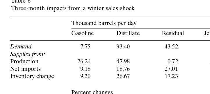
Table 6
Three-month impacts from a winter sales shock Thousand barrels per day
Gasoline Distillate Residual Jet fuel Other
Demand y7.75 93.40 43.52 y2.99 y4.80
Supplies from:
Production y26.24 47.98 y0.72 y31.06 y51.87
Net imports 9.18 18.76 27.01 10.69 y8.13
Inventory change 9.30 26.67 17.23 17.38 55.19
Percent changes Prices
Spot 1.62 1.67 y0.42 0.92 NA
Futures 1.58 1.33 y0.42 0.79 NA
Import 1.27 1.16 y0.31 0.68 NA
Demand y0.10 2.71 4.53 y0.19 y0.12
roughly 50% of distillate sales, is sensitive to home heating requirements in the northeastern United States. The single largest market for residual fuel oil is electric power generation, which is sensitive to heating demands and air condition-ing loads. The other three products decline negligibly. Hence, we focus our discussion on distillate and residual fuel oil markets.
The main purpose of this simulation is to determine how these sales shocks are supplied. Do refiners supply these unanticipated demands from current production, from inventory supplies, or from imports of refined products? Of the 93 thousand
Ž .
barrels per day tbd increase in distillate sales, more than half is from higher
Ž .
production see Table 6 . Additional supplies come from a combination of higher
Ž .
net imports 19 tbd and an inventory drawdown of nearly 27 tbd. These results suggest considerable flexibility in current production to meet sales shocks. Never-theless, supplies flowing from inventory and net imports are important. Petroleum refiners seem to be employing a flexible strategy for dealing with distillate fuel oil sales shocks drawing from each of three major sources of supply.
Another interesting finding is that the cold weather shock induces a price backwardation, defined when spot prices rise above prices for future delivery. Notice in Table 6 that the percentage increase in spot prices for distillate is greater than the percentage increase in distillate futures prices. This finding is important
Ž .
because the study by Williams and Wright 1991 argues that commodity price backwardations arise from stockouts when producer inventories disappear. Our simulations illustrate that price backwardations arise because producer returns to stock holding rise with sales.
The simulation results for residual fuel also tell an interesting story. Nearly all-additional supplies come from increases in net imports and inventory depletion
Table 7
Three-month impacts from a crude oil price shock Thousand barrels per day
Gasoline Distillate Residual Jet fuel Other
Supplies from:
Production 7.29 y10.70 1.92 y0.78 2.89
Net imports 9.92 6.55 0.60 2.18 3.58
Inventory change y17.21 4.14 y2.52 y1.39 y0.76
Percent changes Prices
Spot 4.87 5.35 8.24 5.92 NA
Futures 4.72 5.59 8.27 5.96 NA
Import 3.90 3.66 6.78 4.45 NA
suggesting that residual imports may serve as a buffer to meet sales shocks. US residual fuel oil markets are unique because several large refineries in the Caribbean region can supply residual fuel on relatively short notice given their proximity to US markets.
We finally simulate the market impacts of a 10% increase in crude oil prices during the winter. As expected, product prices increase. By construction, product sales are unchanged because we do not include the sales functions in the model
Ž .
simulation. Net imports for all products increase see Table 7 because we implicitly assume foreign producers do not face the same increase in crude oil
Ž .
prices. Refinery inputs and stocks of crude oil not shown in Table 7 decline. Consequently, producers draw down raw material inventories when input prices rise, consistent with cost smoothing.
With the exception of distillate fuel oil, supplies from product inventories
Ž .
decline see Table 7 . There are two opposing forces affecting product inventory levelsᎏproduction levels and user costs. Our econometric estimates indicate that stocks rise with higher production for all products and fall with increased user costs for all products except residual fuel oil. User costs, which are endogenous in the model, increase for all inventories except distillate in this simulation. Distillate stocks decline because imports increase, which lowers required production and inventory levels. These results suggest that producers may employ different strate-gies to meet sales and cost shocks, depending upon access to imports, transport costs, and other logistical factors.
References
Bacon, R., Chadwick, M., Dargay, J., Long, D., Mabro, R., 1980. Demand, Prices, and the Refining Industry. Oxford Institute for Energy Studies, Oxford, England.
Considine, T.J., 1992. Refined product supply module for EIA’s short-term integrated forecasting
Ž .
system version III SFIFS-III . The Washington Consulting Group, August, 33 pp.
Considine, T.J., 1997. Inventories under joint production: an empirical analysis of petroleum refining. Rev. Econ. Stat. LXXIX, 493᎐502.
Considine, T.J., 1998. Markup pricing in a short-run model with inventories. The Pennsylvania State University, Center for Economic and Environmental Risk Assessment.
Considine, T.J., Larson, D.F., 1998. Uncertainty and the convenience yield in crude oil price backwarda-tions. The Pennsylvania State University, Center for Economic and Environmental Risk Assessment. Davison, R., MacKinnon, J.G., 1993. Estimation and inference in econometrics. Oxford University
Press, New York, NY.
Energy Information Administration, 1993. Short-term integrated forecasting system: 1993 model docu-mentation report. Office of Energy Markets and End Use, US Department of Energy, Washington,
Ž .
D.C., DOErEIA-M041 93 .
Epstein, L.G., Denny, M.G.S., 1983. The multivariate flexible accelerator model. Its empirical
restric-Ž .
tions and an application to US manufacturing. Econometrica 51 3 , 647᎐674.
Griffin, J.M., 1976. The econometrics of joint production: another approach. Rev. Econ. Stat. 59, 389᎐397.
Hansen, L.P., 1982. Large sample properties of generalized method of moments estimators. Economet-rica 50, 1029᎐1054.
Heo, E., 1998. Short-run analysis of market shocks to energy prices: a case of the US petroleum refining
Ž .
industry. J. Korean Inst. Mineral Energy Resour. Eng. 35 1 , 96᎐102.
Hylleberg, Engle, R.F., Granger, C.W.J., 1990. Seasonal integration and cointegration. J. Econometrics 44, 215᎐238.
Kamien, M.I., Schwartz, N.L., 1991. Dynamic Optimization: The Calculus of Variations and Optimal Control in Economics and Management. North-Holland, New York, NY.
Lucas, R., 1967. Optimal investment policy and the flexible accelerator. Int. Econ. Rev. 78᎐85. Luh, Y., Stefanou, S.E., 1996. Estimating dynamic dual models under nonstatic expectations. Am. J.
Ž .
Agric. Econ. 78 4 , 991᎐1003.
Mahmud, S.F., Robb, A.L., Scarth, W.M., 1986. On estimating dynamic factor demands. J. Appl. Econometrics 2, 69᎐75.
McLaren, K., Cooper, R., 1980. Intertemporal duality: application to the theory of the firm. Economet-rica 48, 1755᎐1762.
Miron, J.A., Zeldes, S.P., 1988. Seasonality, cost shocks, and the production smoothing model of inventories. Econometrica 56, 877᎐908.
Newey, W.K., West, K.D., 1994. Automatic lag selection in covariance matrix estimation. Rev. Econ. Stud. 61, 631᎐653.
Ž .
Pindyck, R.S., 1994. Inventories and the short-run dynamics of commodity prices. Rand J. Econ. 25 1 , 141᎐159.
Stefanou, S.E., 1989. Returns to scale in the long-run: the dynamic theory of cost. South. Econ. J. 55, 570᎐579.
Stefanou, S.E., Fernandez-Cornejo, J., Gempesaw II, C.M., Elterich, J.G., 1992. Dynamic structure of production under a quota: the case of milk production in the Federal Republic of Germany. Eur. Rev. Agric. Econ. 19, 283᎐299.
Treadway, A., 1971. The rational multivariate flexible accelerator. Econometrica 39, 845᎐856. Williams, J.C., Wright, B.D., 1991. Storage and Commodity Markets. Cambridge University Press,