Directory UMM :Data Elmu:jurnal:A:Atmospheric Research:Vol55.Issue3-4.2000:

(1)

Ž .

Atmospheric Research 55 2000 225–255

www.elsevier.comrlocateratmos

A bin-microphysics cloud model with high-order,

positive-definite advection

Alexandre A. Costa

a,b,)

_{, Gerson P. Almeida}

b

_,

Antonio Jose C. Sampaio

ˆ

´

b,1

a

Department of Atmospheric Science, Colorado State UniÕersity, Fort Collins, CO, USA

b

Laboratorio de Fisica de NuÕens e, Departamento de Fısica, Uni´ Õersidade Federal do Ceara,´

Fortaleza, CE, Brazil

Received 30 March 1999; received in revised form 2 June 2000; accepted 7 September 2000

Abstract

An axisymmetric, anelastic model of a convective cloud is described. The model comprises prognostic equations for the azimuthal vorticity, the perturbation potential temperature, the perturbation water vapor mixing ratio, 44 categories of cloud condensation nuclei, and 100 categories of liquid-phase hydrometeors. Results from a control simulation show that the model is capable to reproduce realistically the life cycle of a convective cloud including the production of warm rain.

A discussion of the role of advection in bin-microphysics models is presented and sensitivity tests were performed regarding the order of advection. The results show that, although the global characteristics of all simulated clouds were similar, significant differences occur with respect to their microstructure, particularly close to the cloud edges, when the order of the advective scheme changes. The conclusion is that intermediate-order advection schemes can indeed be used in cloud-resolving simulations, as far only as the gross characteristics of the cloudrcloud system are being investigated, but not poor, low-order schemes. On the other hand, the sensitivity with respect to the advection suggests that the evaluation of cloud phenomena that occur in fine-scales, such as entrainment and certain microphysical and radiational processes, must require the use of accurate, higher-order schemes.q_{2000 Elsevier Science B.V. All rights reserved.}

Keywords: Bin-microphysics cloud model; Advection; Simulation

)_{Corresponding author. Tel.:}_q_{55-85-288-9904; fax:}_q_{55-85-288-9903.}

Ž .

E-mail address: [email protected] A.A. Costa .

1

Ž .

(2)

( ) A.A. Costa et al.rAtmospheric Research 55 2000 225–255

226

1. Introduction

In the past three decades, many efforts have been made to develop and use cloud

Ž

models. From the early models of dry convection to the modern bin-microphysics e.g.,

. Ž

Kogan, 1991; Reisin et al., 1996, etc. and mesoscale models e.g., Pielke et al., 1992;

.

Xue et al., 1995 , too much progress has been made. For instance, the representation of physical processes, such as turbulence, microphysics, radiation, and surface fluxes, became more and more sophisticated.

Nevertheless, one should point out that atmospheric modeling in mesoscale and cloud-scale did not incorporate, in most cases, the latest developments on numerical techniques, for instance, modern advection schemes. In several current atmospheric

Ž . Ž

models, old and inaccurate numerical schemes are still used see, for instance,

.

Schlunzen, 1994; Christensen et al., 1997; Cox et al., 1998 . Of course, the introduction

¨

of new techniques in very complex models is not always timely, because it is not often clear if one gains more in accuracy than looses in computational cost. Also, changes in complicated models are not usually an easy task.

New numerical schemes can be tested in simple models with ease. Therefore, simple, low-dimension models can still be useful to simulate some specific phenomena as well as to test physical parameterizations andror numerical schemes.

In this paper, a two-dimensional, axisymmetric cloud model containing a warm-phase

Ž

bin-microphysics is presented. Although similar models exist in the literature e.g.,

.

Soong, 1974; Takahashi, 1975; Tzivion et al., 1994 , the present model uses more

Ž

accurate numerical techniques for advection Bott, 1989a,b; Easter, 1993; Costa and

.

Sampaio, 1997 . One of the purposes of this paper, along the description of the model itself, is to explore sensitivities regarding the advection schemes.

In Sections 2–4, the main characteristics of the model are described. In Section 5, results from a control simulation of a deep, isolated, tropical convective cloud are shown. Section 6 is dedicated to a discussion on the use of advective schemes in cloud models. Section 7 shows results from sensitivity tests using the cloud model, regarding the order of advection. In Section 8, an overall discussion is presented.

2. Basic equations

The present model is axi-symmetric, vorticity based, and anelastic, as those described

Ž . Ž . Ž .

by Soong and Ogura 1973 , Soong 1974 , Costa and Sampaio 1996 and Almeida et

Ž .

al. 1998 .

Ž .

The set of basic equations comprises a diagnostic equation for the streamfunction 1 ,

Ž .

and prognostic equations for the azimuthal vorticity 5 , the perturbation potential

Ž . Ž .

temperature 6 , the perturbation water vapor mixing ratio 7 , 44 categories of cloud

Ž . Ž .

condensation nuclei 8 , and 100 categories of liquid-phase hydrometeors 9 . All symbols are listed in Appendix A.

E 1 Ec 1 E2c

q ₂sz,

Ž .

1

ž /

(3)

( )

A.A. Costa et al.rAtmospheric Research 55 2000 225–255 227

where experiments performed in this paper, the subgrid-scale transport terms of CCNs and cloud droplets were set to zero, in order to emphasize the model sensitivity to the numerical diffusion associated with the advection schemes.

3. Microphysics

(4)

228

CCN are activated as the supersaturation exceeds the critical value determined by Kohler’s curve. Because only the small nuclei reach their equilibrium size rapidly

¨

Ž_{Mordy, 1959 , the procedure proposed by Kogan 1991 is used to determine the radius}. Ž .

of the activated nuclei at the cloud base, i.e., only small aerosol particles are assumed to reach its equilibrium size.

Ž .

Condensational growth is calculated according to Mordy 1959 . The solute term is

Ž .

calculated only for nuclei at a single microphysical timestep see Section 4 and the

Ž .

curvature term is neglected for raindrops radius greater than 50 mm . The amount of

Ž .

condensedrevaporated water CyE term in Eqs. 6 and 7 and the latent heat released

are calculated based on d rird t.

Changes due to collision–coalescence, collision-breakup and spontaneous breakup are also considered. Coalescence and collisional breakup probabilities are calculated

Ž .

according to Low and List 1982a . Filament, sheet and disk breakup are represented,

Ž .

according to the formulas by Low and List 1982b for the distribution-function of droplet fragments. Spontaneous breakup is incorporated, following a procedure similar

Ž .

to the one proposed by Srivastava 1971 , but with formulas derived from more recent

Ž .

experiments Kamra et al., 1991 .

4. Numerical procedure

In the present version of the cloud model, advection is usually evaluated using the

Ž . Ž . Ž

Area-Preserving Flux-Form APF scheme Bott, 1989a,b . Options from zero-th which

.

is equivalent to the common forward-upstream scheme to eight-order polynomials in

Ž .

the APF advection scheme are available, as in Easter 1993 and Costa and Sampaio

Ž1997 , with distinction to the third- and fifth-order schemes. In the control simulation,. Ž .

the fifth-order scheme APF5 is used.

Ž .

An iterative solver Stone, 1968; Jacobs, 1972 is used to calculate the streamfunction from the vorticity.

Ž .

A simple first-order closure Smagorinsky, 1963 is used in turbulence

parameteriza-Ž .

tion, with turbulent coefficients calculated as in Soong and Ogura 1973 . The same value of those coefficients was used for both the transport of momentum and scalars

Žwith the exception of the distribution-function of drops ..

Cloud condensation nuclei are divided into 44 categories, with dry radii ranging from approximately 0.006 to 7.59 mm and critical supersaturations ranging from almost 0

Žlargest nuclei to 2.8% smallest nuclei . Six out of the 44 categories generate CCN. Ž .

with a moist radius greater than 10mm at the cloud base, although at small

concentra-Ž y1 _.

tions less than 12 l for categories 39 to 44 . The present microphysical model also comprises a set of 100 discrete bins, in which the liquid-phase hydrometeors are categorized, according to their radius, which varies exponentially from 1mm to 5 mm.

Ž

Since microphysical processes condensational growth, collision–coalescence, and

.

break-up alter the distribution-function of drops, mass has to be redistributed among the

Ž .

(5)

( )

Ž .

this method is adopted, as in Kogan 1991 . It can be shown that such an approach reduces drastically the errors associated with the Kovetz–Olund method, and provides realistic values of supersaturation.

Ž .

The large, dynamical timestep Dt is divided into small microphysical timesteps

ŽDt.. For a given variable, the dynamical tendency changes due to resolved advectionŽ .

and subgrid-scale transport is assumed to be uniform within a large timestep, while microphysical tendencies are calculated in each small timestep.

All boundaries are rigid, free-slip. To avoid numerical instabilities, absorbing layers are imposed at the top and lateral boundaries.

5. Control simulation

The domain of integration contains 80=80 grid points with a 120-m grid spacing in both the horizontal and vertical directions and a dynamical timestep of 5 s. A total of 32 absorbing layers was used in both directions.

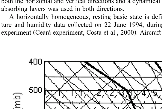
A horizontally homogeneous, resting basic state is defined from upper-air tempera-ture and humidity data collected on 22 June 1994, during a cloud-microphysics field

Ž .

experiment Ceara experiment, Costa et al., 2000 . Aircraft data was not available above

´

Fig. 1. Skew-T diagram depicting the basic state of temperature and dew-point temperature used in the cloud simulations. The sounding was obtained blending the 22 June 1994, 1200Z NCEP analysis over Mossoro,´

(6)

230

3000 m, therefore, they were blended with the NCEP analysis for 12 UTC. The skew-T diagram for the blended sounding is depicted in Fig. 1. The lifting condensation level,

Ž .

the level of free convection and the equilibrium level were found at 910 mb 975 m ,

Ž . Ž .

850 mb 1565 m and 635 mb 3970 m , respectively. As discussed by Sampaio et al.

Ž_{1996 and Costa et al. 1998 , those atmospheric conditions favored the formation of}. Ž .

precipitating warm cumuli.

The nuclei are assumed to be composed by NaCl only. The total nucleus concentra-tion is assumed to be constant below 500 m. Above that level, the concentraconcentra-tion decays exponentially with height.

Convection was triggered, introducing a warm bubble with a maximum perturbation potential temperature of 1 K, in which the relative humidity was increased by 5%.

Fifth-order APF advection is adopted for the control run. Flux correction is imposed to the advection of CCN and hydrometeors.

Table 1 shows some parameters for the simulated cloud and compares them with actual observations. The modeled values in Table 1 are physically reasonable and some

Ž .

of them droplet concentration, cloud base and top heights are in good agreement with observations from a warm, precipitating cumulus cloud that was penetrated in five different levels, on 22 June 1994, during the Ceara experiment.

´

Figs. 2–4 show snapshots of the simulated cloud for 10, 18, and 24 min, correspond-ing roughly to its growcorrespond-ing, mature, and precipitatcorrespond-ingrdecaying stages, respectively. Fig. 5 shows the time evolution of selected fields at the central axis of the cloud.

During the early stages, the cloud top rises at a ratio of about 3 msy1_{, which is less}

than the maximum vertical velocity found at the major cloud updraft.

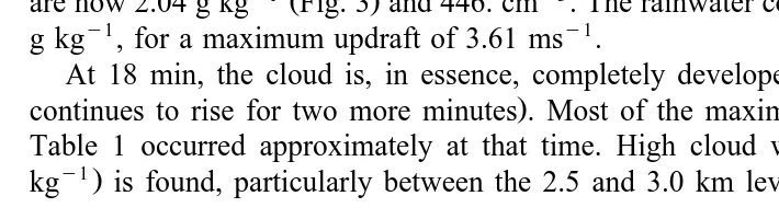
At 10 min, the cloud expanded, with its top reaching 2.8 km for a horizontal dimension of about 5 km. The maximum cloud water content and droplet concentration

y1 _Ž _. y3

are now 2.04 g kg Fig. 3 and 446. cm . The rainwater content is still less than 0.01 g kgy1_{, for a maximum updraft of 3.61 ms}y1_.

Ž

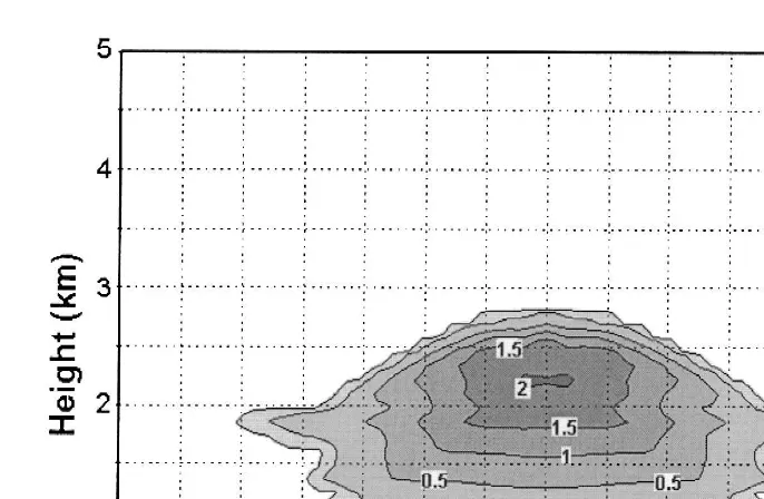
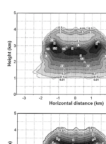
At 18 min, the cloud is, in essence, completely developed although the cloud top

.

continues to rise for two more minutes . Most of the maximum field values shown in

Ž

Table 1 occurred approximately at that time. High cloud water mixing ratio )3 g

y1_. _Ž _.

kg is found, particularly between the 2.5 and 3.0 km levels Fig. 4a . In the upper

Table 1

Ž .

Some physical characteristics of the simulated cloud control run , compared with observations

Parameter Modeled value Observed value

Maximum cloud water mixing ratio g kg 3.99 1.2

y1

Ž .

Maximum rainwater mixing ratio g kg 6.54 3.1

y3

Ž .

Maximum droplet number concentration cm 563 541

Ž .

Maximum cloud top height mb 623 720

Ž .

Minimum cloud base height mb 904 908

y1

Ž .

(7)

( )

Ž .

Fig. 2. Cloud water mixing ratio of the simulated cloud control run, 10 min of simulation .

portion of the cloud, the cloud water content was significantly depleted, due to the

Ž . Ž

conversion to rainwater Fig. 4b . The greatest value of the droplet concentration 563

y3 _.

cm , see Table 1 occurred 2 min before; however, a significant portion of the cloud

Žright above the cloud base is still filled with number concentrations greater than 500.

y3 y1_Ž

cm . A few points exhibit values of rainwater mixing ratio greater than 6 g kg Fig.

. Ž

4b ; however, the drops are still not able to overcome the strong updraft upward winds

y1 _.

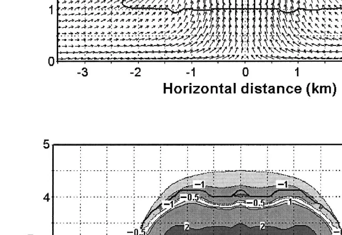
with speeds close to 5 ms occupy significant portions of the cloud, as seen in Fig. 4c . The structure of the perturbation potential temperature is depicted in Fig. 4d, where the heating associated with the condensation process produced departures from the basic state greater than 3.5 K. On the other hand, evaporative cooling at the cloud top generated negative perturbations with absolute values greater than 2 K.

Both the liquid water fields and the cloud extension drop, as the end of simulation approaches. At 24 min, the maximum cloud water mixing ratio was reduced to 0.73 g

y1 _Ž _. y3

kg Fig. 5a , and the maximum droplet concentration dropped down to 321 cm .

Ž

The water field is now dominated by raindrops maximum rainwater mixing ratio of

y1_.

(8)

232

Ž . Ž . Ž .

Fig. 3. Cloud water mixing ratio a , rainwater mixing ratio b , perturbation potential temperature c , and

Ž . Ž . Ž .

wind vectors d for the simulated cloud control run, 18 min of simulation . The thick black line in panels b ,

Ž . Ž . y1

(9)

( )

Ž .

(10)

234

Ž . Ž . Ž

Fig. 4. Cloud water mixing ratio a , and rainwater mixing ratio b for the simulated cloud control run, 24

.

(11)

( )

Ž . Ž .

Fig. 5. Time evolution of the cloud water mixing ratio a , and rainwater mixing ratio b at the central axis of

Ž .

(12)

236

Ž .

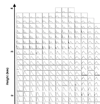
Fig. 6. Cloud droplet spectra of the simulated cloud APF5rcontrol run, 18 min of simulation . The abscissa corresponds to the droplet radius, ranging from 0 to 50mm. The scale is linear. The ordinate is the number concentration correspondent to each bin. The scale is logarithmic, ranging from 0.1 to 100 cmy3_.

clouds, in general, and with the ones made during the Ceara experiment, in particular.

´

Close to the cloud boundaries, and especially at its top, bi- and multimodal spectra occurred. In the upper kilometer of the cloud, bimodal spectra are, in fact, dominant.

6. Cloud modeling and advection schemes

(13)

( )

diffusion, or negative values for an expected positive-definite quantity. For instance, the simple upstream, forward-in-time scheme, produces a very significant damping, while the very popular leapfrog scheme, despite being amplitude-preserving, produces spuri-ous oscillations and phase errors.

Ž .

As shown by Tremback et al. 1987 , high-order advection can reduce the numerical diffusion dramatically. On the other hand, flux correction can provide oscillation-free

Ž . Ž .

solutions e.g., Smolarkiewicz, 1984; Bott, 1989a,b . Costa and Sampaio 1997 showed that a high-order positive-definite scheme could indeed be useful to obtain very accurate solutions for the advection equation.

The weak development of numerical techniques and the lack of understanding on the role of advection schemes in cloud modeling led early cloud modelers to use simple

Žand poor schemes. The most popular scheme during the 1970s was certainly the.

Ž .

forward-upstream e.g., Ogura and Takahashi, 1971; Soong and Ogura, 1973 , but other

Ž .

modelers used the leapfrog scheme e.g., Murray and Koenig, 1972 or other simple algorithms.

Ž

As more accurate numerical schemes were developed e.g., Purnell, 1976; Arakawa

.

and Lamb, 1981; Smolarkiewicz, 1984; Bott, 1989a , they were being incorporated into atmospheric models. In recent cloud modeling studies, many authors adopted positive-definite schemes, particularly if bin-microphysics schemes are present. For instance,

Ž . Ž .

Brenguier and Grabowski 1993 used the scheme proposed by Smolarkiewicz 1984

Ž .

and Smolarkiewicz and Grabowski 1990 to investigate entrainment as simulated by a

Ž .

two-dimensional bin-microphysics cloud model. Feingold et al. 1994 used sixth-order

Ž .

polynomial fitting Tremback et al., 1987 , plus flux renormalization and

positive-defi-Ž .

nite constraints Bott, 1989b in large-eddy simulations of stratocumulus clouds. One of the first articles addressing the importance of advection in cloud modeling

Ž .

was presented by Orville and Sloan 1970 , hereafter referred to as OS. They verified the influence of different orders of advection in a two-dimensional model of orographic clouds, comparing results obtained with the standard, first-order, forward-upstream

Ž .

scheme, and Crowley’s 1968 second- and fourth-order schemes. Their results show that, for a symmetric case with no ambient wind, the three schemes produced similar results. Because in their kinetic energy analysis, the truncation error associated with the forward-upstream scheme was found to be significant, and since the second-order Crowley’s scheme is obviously superior to the fourth-order scheme in terms of computa-tional efficiency, the authors recommend the use of the second-order scheme for advection. The results shown in the next section of this manuscript are in agreement with some of the conclusions by OS. In particular, as far as the model resolution is fine enough to resolve the cloud using a large number of grid points, the advective scheme is not very important to determine the gross structure of the cloud. However, this does not guarantee that the advection cannot influence other aspects of the cloud, such as its microstructure.

In multidimensional, non-linear, atmospheric modeling, non-linear interactions, alias-ing and source terms often produce shortwave features. When clouds are present, no matter how small is the grid spacing, the issue of the short modes is even more

Ž .

(14)

238

Ž .

discontinuities in the water field that often present sharp edges , atmospheric simula-tions involving clouds are necessarily rich in AshortwaveB constituents. This must be even more severe in bin-microphysics models, in which the water is partitioned into a large number of components. Therefore, because those shortwave features are a problem for most numerical schemes, no matter what resolution is used, cloud models in general and bin-microphysics models in particular must have uncertainties with the representa-tion of the water fields, at least at the cloud boundaries. In particular, low-order advection schemes, for which the representation of the phase and amplitude of narrow modes is poor, are probably not suitable for cloud simulations in which cloud-edge processes, such as entrainment, are being investigated, especially if a bin-microphysics is present. Because OS used a very simplified bulk-microphysics parameterization, they could not discuss this issue properly.

In order to check this hypothesis, the role of the order of the advective scheme is

Ž

investigated in the context of a non-linear model cloud model described in Sections

.

2–4 . In the next section, results from sensitivity experiments using different advection

Ž .

schemes are presented. The schemes are the standard forward-upstream FWD , and

Ž .

three other versions of the area-preserving flux-form advection scheme APF .

FWD advection is widely described in the literature. It uses forward-in-time, upwind-in-space differencing, and produces a very strong damping, particularly for short wavelengths. Due to its severe limitations, FWD was practically abandoned in cloud

Ž

modeling, however, because it can be treated as theAzero-th orderB APF algorithm see

.

Bott, 1989a; Easter, 1993 , it is going to be used in this paper to illustrate the extreme low-order case of area-preserving positive-definite advection. The APF scheme,

pro-Ž .

posed by Bott 1989a,b , is positive-definite, and presents both small phase and

Ž

amplitude errors. Like many other advection algorithms e.g., Crowley, 1968; Tremback

.

et al., 1987 , the APF scheme uses polynomial fitting to represent a given variable within a grid box. A detailed description of the APF scheme can be found in Bott

Ž1989a,b or Chlond 1994 . In this study, second-order APF2 , modified using the. Ž . Ž . Ž

. Ž . Ž .

terminology by Easter, 1993 third-order APF3 , and modified fifth-order APF5 versions of the scheme are going to be used. Coefficients for APF2, APF3, and APF5

Ž . Ž . Ž .

are given according to Bott 1989b , Easter 1993 and Costa and Sampaio 1997 ,

Ž .

respectively. It can be shown that FWD orAAPF0B , APF2, APF3 and APF5 provide first-, third-, fourth- and sixth-order accuracy in space, respectively. The shortcomings due to the first-order accuracy in time for a time-varying wind field are not important because of the small timestep used in this study.

7. Sensitivity tests regarding the advection scheme

Sensitivity tests regarding the advection scheme were performed, using the cloud model described in previous sections. In order to compare the performance of the different advection schemes in the context of the cloud model, the ambient and initial conditions, as well as all numerical settings used in the control simulation, were preserved, with the only exception of the advection algorithm. In three sensitivity tests,

Ž .

(15)

( )

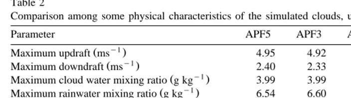
A.A. Costa et al.rAtmospheric Research 55 2000 225–255 239 Table 2

Comparison among some physical characteristics of the simulated clouds, using different advection schemes

Parameter APF5 APF3 APF2 FWD MIX

y1

Ž .

Maximum updraft ms 4.95 4.92 4.84 5.19 4.99

y1

Ž .

Maximum downdraft ms 2.40 2.33 2.19 1.83 2.46

y1

Ž .

Maximum cloud water mixing ratio g kg 3.99 3.99 3.95 4.34 4.04

y1

Ž .

Maximum rainwater mixing ratio g kg 6.54 6.60 6.65 8.10 7.64

y3

Ž .

Maximum droplet number concentration cm 563 553 536 674 503

Ž .

Maximum cloud top height mb 623 623 623 627 623

Ž .

Minimum cloud base height mb 904 904 904 917 904

y1

Ž .

Maximum precipitation rate mm h 10.2 10.4 10.6 7.1 5.5

Ž . Ž . Ž . Ž .

fourth APF3 , third APF2 and first FWD . In the last sensitivity run MIX , APF5 advection was used for all fields, except for the distribution-function of drops, advected according to the forward-upstream scheme. The purpose of MIX was to investigate the effect of low-order advection on the liquid water field only, providing a more direct comparison to APF5.

The global characteristics of the life cycle of the simulated cloud were not very sensitive to the change in the advection scheme. Table 2 compares some parameters of

Ž .

the five simulated clouds controlrAPF5, APF3, APF2, FWD, and MIX . Both the vertical and horizontal dimensions of the simulated clouds were very similar. The most significant departures from the control simulation occurred regarding the maximum rainwater content, which was higher in the FWD cloud, and the maximum compensating downdraft, which decreased as the order of advection decreased. Surprisingly, the FWD run showed the greatest updraft. Both sensitivities can be possibly explained by changes in the transport of the vorticity field. In particular, if a highly diffusive scheme is used, vorticity is diffused radially. Eventually, a tail of positive values in the vorticity field

Žthat generates the downdraft leaves the effective model domain determined by the. Ž .

absorbing layers . As one integrates the vorticity inward, to obtain the velocity field, the loss of positive vorticity not only weakens the downdraft, but also may produce a stronger updraft at the center of the domain, even with an increased dissipation of kinetic energy. Hence, one should not expect this result to be general; it is probably geometry- and model-dependent.

Despite the similarities in the gross structure of the simulated clouds, the fine structure of the cloud exhibits important sensitivities. In particular, the sensitivity tests suggest that both dynamical and microphysical processes at cloud edges can be significantly influenced by the choice of the advection scheme.

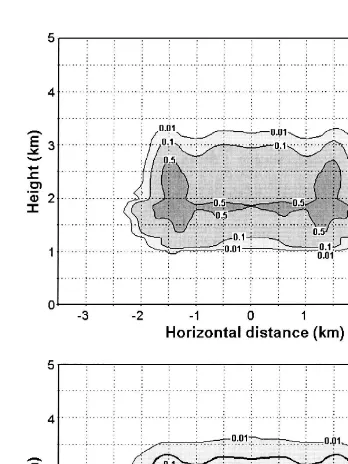
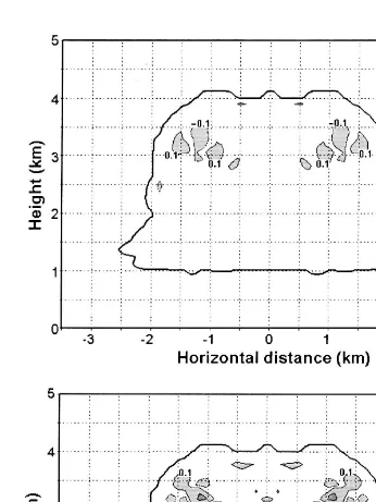
In fact, the greatest departures among the simulated clouds occur at the cloud edges, as shown in Figs. 7–10. The different frames depict the departure of the cloud water

Ž . Ž . Ž .

content a , rainwater content b , perturbation potential temperature c and wind

Ž . Ž . Ž

vectors d between the control run and the simulations using APF3 Fig. 7 , APF2 Fig.

. Ž . Ž .

8 , FWD Fig. 9 and MIX Fig. 10 .

The differences between the APF5 and APF3 clouds are, in general, small. Close to the cloud top, the departures at the cloud water and rainwater fields are mostly of the

y1 _Ž _.

(16)

240

Ž . Ž .

Fig. 7. Differences in the cloud water mixing ratio a , rainwater mixing ratio b , perturbation potential

Ž . Ž . Ž

temperature c and wind vectors d between the APF3 and the APF5rcontrol simulations 18 min of

. y1

(17)

( )

Ž .

Fig. 7 continued .

Ž .

temperature field occurred at the cloud top and were less than 0.5 K Fig. 7c . Differences at the eddy structure were also small and were present primarily at the cloud

Ž .

(18)

242

The fields in the simulation in which APF2 was used depart more from the control run, as expected. Differences greater than 0.5 g kgy1 in the cloud water mixing ratio

Ž . y1 _Ž _.

Fig. 8a and greater than 2.0 g kg in the rainwater mixing ratio Fig. 8b were

Ž .

(19)

( )

Ž .

(20)

244

Ž .

verified. Close to the cloud top, temperature departures greater than 1 K Fig. 8c and significant discrepancies in the simulated wind field were present.

The largest departures from the control run were observed in the simulation using

Ž y1_.

FWD. Large differences in the cloud water field greater than 1.0 g kg were

Ž .

(21)

( )

Ž .

observed in several portions of the cloud, about the level where the maximum rainwater

Ž .

was attained at the control run Fig. 9a . In addition, the FWD cloud showed an excess of more than 3 g kgy1

at the central axis and a deficit of more than 1 g kgy1

off the

Ž .

(22)

246

Ž .

(23)

( )

Ž .

use of a highly diffusive scheme has significant influence on the process of precipitation

Ž .

development. Very large departures occurred in both the temperature Fig. 9c and wind

(24)

248

simulations, for which the differences from the control run were primarily found at the cloud borders, in the FWD simulation they were present throughout the entire cloud.

The structure of the water field in MIX resembled the one in the FWD run, with differences from the control simulation greater than 2 g kgy1 in the cloud water mixing

Ž . y1 _Ž _.

ratio Fig. 10a and greater than 3 g kg in the rainwater mixing ratio Fig. 10b . The major differences in the temperature and wind fields between MIX and APF5 occurred

Ž .

at the cloud edges mostly top and lateral boundaries , due to the influence of the advective schemes on the transport of droplets in those regions.

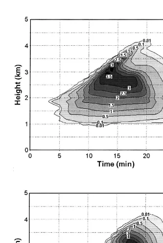
Because the difference in the accuracy of the advective schemes has more influence in the cloud edges, it induces important changes in the cloud microstructure. One important example is the change in the occurrences of bi- and multimodal spectra. As shown in Fig. 11, as the order of the advection scheme increases, there is a general tendency for the bi- and multimodal droplet spectra to become more frequent. This is probably due to the improved representation of the sharp discontinuities in the dynamic, thermodynamic and water fields at the cloud borders by higher-order schemes. The differences are very significant, even considering the APF5 and APF3 runs. In Fig. 11, it is also noticeable that when the FWD scheme is used for the advection of hydrometeors, the number of bi- and multimodal distributions reaches its maximum at a later time.

Fig. 12 shows the evolution of the rainwater mixing ratio at the gridbox closest to the surface and to the domain’s central axis for the five runs. The results from APF5, APF3

(25)

( )

Fig. 12. Time dependence of the rainwater mixing ratio at the lowest gridpoint at the central axis of the cloud

Žzs60 m, rs60 m ..

and APF2 are very similar this time. Despite the difference in the amplitude, they show very peaked rain events, with a maximum at 25 min. In the FWD and MIX runs, the rainwater mixing ratio peaks 1 min later and the precipitation event lasts longer, probably due to a spurious diffusive transport of drops in the vertical. Supposedly, the different types of precipitation evolution are also associated with the different patterns in spectrum broadening shown next.

In order to illustrate how the choice of the order of advection can alter the statistical properties of the droplet spectra, Fig. 13 depicts the standard-deviation of the diameter

Ž .

of the cloud droplets normalized by the mean after 18 min of simulation, along with the corresponding observed field. In all runs, immediately above the cloud base, the normalized standard deviation tends to decrease, suggesting that droplet growth by condensation dominates in that region. Between 0.5 and 1.0 km above the cloud base, this tendency reverses, and the spectra tend to become broader, possibly due to significant growth via collision–coalescence. Above 3 km, the normalized diameter

Ž .

standard deviation increases sharply at least in simulations APF5, APF3 and APF2 . As shown in Fig. 6, this is the region corresponding to the dominance of bimodal spectra. The most significant differences from the APF5 simulation in Fig. 13 are associated

Ž .

(26)

250

Fig. 13. Lines: normalized diameter standard deviation at the cloud’s central axis as a function of height for

Ž .

the control and sensitivity runs 18 min of simulation . Dots: Observed normalized diameter standard deviation

Ž .

(27)

( )

spectra in those two simulations were broader than the ones in APF5 at the lower portion of the cloud. On the other hand, the normalized diameter standard deviation in FWD and MIX does not present the sharp peak found in the other three simulations. Although there is some influence of the different AtimingB in the microphysical evolution of those two clouds, in comparison to the other three, this is mostly associated with the smaller number of bi- and multimodal spectra in FWD and MIX. Due to the same reason, the peak relative to the APF2 simulation is less pronounced. It is clear that the agreement between the observed and modeled normalized diameter standard devia-tion is greater when higher-order advecdevia-tion schemes were used.

Finally, in order to illustrate how the use of more diffusive schemes alter the actual shape of the drop spectra, the distribution-function of drops for the MIX simulation is shown in Fig. 14. The comparison with Fig. 6 shows some clear differences.

Ž .

(28)

252

Ž .1 Due to the numerical diffusion of drops, at the outflow region above 2.5 km , theŽ .

boundaries of the MIX cloud often extend beyond the contour of the APF5 cloud, reducing the gradients in those regions. Because the thermodynamic field, particularly at the cloud top, depends strongly on the evaporation of the water particles, the most pronounced temperature differences between MIX and APF5 occurred in that region. As a consequence, the most striking differences in the wind field were also located by the cloud top.

Ž .2 There are less grid boxes containing multiple modes in Fig. 14 than in Fig. 6, in agreement with what was stated previously.

Ž .3 There is a less dramatic mode separation in the upper grid boxes in Fig. 14 than in Fig. 6, causing the reduction in the normalized diameter standard deviation at the upper portion of the cloud, from APF5 to MIX, shown in Fig. 13.

Ž .4 The MIX cloud Fig. 14 exhibits relatively broad spectra in its mid and lowerŽ . Ž .

portions, in contrast with the narrower spectra found in the APF5 cloud Fig. 6 . Again, this is in agreement with what was shown in Fig. 13.

8. Summary, concluding remarks, and future work

A two-dimensional cloud model, conceived to simulate deep, isolated convective cells is presented, in which a warm, bin-microphysics representing multiple processes

Žnucleation, condensationrevaporation, coalescence, collisional and spontaneous breakup

.

and sedimentation and an accurate, positive-definite advection scheme are used. Despite the limitations regarding the lack of the third degree of freedom and the assumption of axisymmetry, the model is capable to simulate realistically several aspects of the evolution of a convective cloud.

The model was able to capture the generation of bi- and multimodal spectra at the cloud boundaries during its mature stage, particularly at the cloud top. The significant variability in cloud spectra, as well as the occurrence of multimodes, suggests that most of the microphysics bulk-parameterizations, based, for instance, on exponential or generalized gamma distributions, cannot represent some important aspects of the mi-crostructure and life cycle of convective clouds.

Sensitivities with respect to the use of different advection schemes were explored. The results show that the gross aspects of the life cycle of the different simulated clouds were similar in all cases, even when a very poor scheme, such as the forward-upstream, was used. It suggests that the ambient and initial conditions are far more important to determine the bulk properties of the simulated clouds.

One should point out, however, that important differences occurred among the simulated clouds, regarding their dynamics, thermodynamics and microphysics, particu-larly at the cloud boundaries. In fact, the use of low-accuracy advection produced important changes in the entire cloud, while the use of intermediate-accuracy advection caused deviations mostly restricted to the cloud edges.

The results suggest that, in fact, low-order advection schemes can be used to simulate

Ž

clouds or cloud systems if one is only interested in their global characteristics gross

.

(29)

( )

is interested in looking at their fine structure, particularly at the microphysics. In the latter case, intermediate-order schemes also have shortcomings, because they still produce poor results close to sharp discontinuities. In this case, although far from being

Ž .

aAperfect solutionB for the problem, high-order schemes such as APF3 or even APF5 are certainly useful. In terms of the statistics of droplet spectra, again a reasonable agreement between observed and modeled fields could only be found when intermediate to high-order advection was used. Those conclusions are expected, since the bulk characteristics of the cloud are dominated by the coarse modes in the model grid. On the other hand, cloud-edge processes, which are very important to the evolution of the cloud

Ž

microphysics and other phenomena, such as the ones associated with radiation, which

.

were not explored in this paper are very much influenced by narrow modes, such as 2D

or 4D features.

Acknowledgements

The authors wish to thank three anonymous reviewers for their valuable contribu-tions. Gerson Paiva Almeida gratefully acknowledges the support received from CAPES

ŽCoordenac

¸

ao de Aperfeic

˜

¸

oamento de Pessoal de Nı

´

Õel Superior ..

u₀ basic state potential temperature

L latent heat of evaporation

qXÕ perturbation water vapor mixing ratio

qÕ₀ basic state water vapor mixing ratio

q_l liquid water mixing ratio

nj category of cloud condensation nuclei

fi category of liquid-phase hydrometeor

t_i turbulent mixing terms

(30)

254

Almeida, G.P., Costa, A.A., Mendes, K.C., Sampaio, A.J.C., 1998. Detailed microphysics in a two-dimen-sional cloud model. Preprints of the AMS Conference on Cloud Physics, Everett, Washington, USA. pp. 91–94.

Arakawa, A., Lamb, V.R., 1981. Potential entrophy and energy conserving scheme for the shallow water equations. Mon. Weather Rev. 109, 18–36.

Bott, A., 1989a. A positive definite advection scheme obtained by nonlinear renormalization of the advective fluxes. Mon. Weather Rev. 117, 1006–1015.

Bott, A., 1989b. Reply. Mon. Weather Rev. 117, 2633–2636.

Brenguier, J.-L., 1993. Observations of cloud microstructure at the centimeter scale. J. Appl. Meteorol. 32, 783–793.

Brenguier, J.-L., Grabowski, W.W., 1993. Cumulus entrainment and cloud droplet spectra: a numerical model within a two-dimensional framework. J. Atmos. Sci. 50, 120–136.

Chlond, A., 1994. Locally modified version of Bott’s advection scheme. Mon. Weather Rev. 122, 111–125. Christensen, J.H., Machenhauer, B., Jones, R.G., Schar, C., Ruti, P.M., Castro, M., Visconti, G., 1997.¨

Validation of present-day regional climate simulations over Europe: LAM simulations with observed boundary conditions. Clim. Dyn. 13, 489–506.

Costa, A.A., Sampaio, A.J.C., 1996. A two-dimensional cloud model: description and numerical experiments. Proceedings of the 12th International Conference on Clouds and Precipitation, Zurich, Switzerland. pp. 782–785.

Costa, A.A., Sampaio, A.J.C., 1997. Bott’s area-preserving flux form advection algorithm: extension to higher orders and additional test. Mon. Weather Rev. 125, 1983–1989.

Costa, A.A., Coelho, A.A., Brenguier, J.-L., de Oliveira, C.J., de Oliveira, J.C.P., 1998. On the variability of microphysical parameters in tropical cumulus clouds. Preprints of the AMS Conference on Cloud Physics, Everett, Washington, USA. pp. 518–521.

Costa, A.A., de Oliveira, C.J., de Oliveira, J.C.P., Sampaio, A.J.C., 2000. Microphysical observations of warm cumulus clouds in Ceara State, Brazil. Atmos. Res. 54, 167–199.´

Cox, R., Bauer, B.L., Smith, T., 1998. A mesoscale model intercomparison. Bull. Am. Meteorol. Soc. 79, 265–283.

Crowley, W.P., 1968. Numerical advection experiments. Mon. Weather Rev. 96, 1–11.

Easter, R.C., 1993. Two modified versions of Bott’s positive definite numerical advection scheme. Mon. Weather Rev. 121, 297–304.

Feingold, G., Stevens, B., Cotton, W.R., Walko, R.L., 1994. An explicit cloud microphysicsrLES model designed to simulate the Twomey effect. Atmos. Res. 33, 207–233.

Jacobs, D.A.H., 1972. The strongly implicit procedure for numerical solution of parabolic and elliptic partial differential equations. Central Electricity Research Laboratory-Note RDrLrN66r72.

Kamra, A.K., Bhalwankar, R.V., Sathe, A.B., 1991. Spontaneous breakup of charged and uncharged water drops freely suspended in a wind tunnel. J. Geophys. Res. 96, 17159–17168.

(31)

( )

A.A. Costa et al.rAtmospheric Research 55 2000 225–255 255 Kovetz, A., Olund, B., 1969. The effect of coalescence and condensation on rain formation in a cloud of finite

vertical extent. J. Atmos. Sci. 26, 1060–1065.

Low, T.B., List, R., 1982a. Collision, coalescence, and breakup of raindrops: Part. 1. Experimentally established coalescence efficiencies and fragment size distributions in breakup. J. Atmos. Sci. 39, 1591–1606.

Low, T.B., List, R., 1982b. Collision, coalescence, and breakup of raindrops: Part 1. Parameterization of fragment size distribution. J. Atmos. Sci. 39, 1607–1618.

Mordy, W., 1959. Computation of the growth by condensation of a population of cloud droplets. Tellus 11, 16–44.

Murray, F.W., Koenig, L.R., 1972. Numerical experiments on the relation between microphysics and dynamics in cumulus convection. Mon. Weather Rev. 100, 717–732.

Ogura, Y., Takahashi, T., 1971. Numerical simulation of the life cycle of a thunderstorm cell. Mon. Weather Rev. 99, 895–911.

Orville, H.D., Sloan, L.J., 1970. Effects of higher order advection techniques on a numerical cloud model. Mon. Weather Rev. 98, 7–13.

Pielke, R.A., Cotton, W.R., Walko, R.L., Tremback, C.J., Lyons, W.A., Grasso, L.D., Nicholls, M.E., Moran, M.D., Wesley, D.A., Lee, T.J., Copeland, J.H., 1992. A comprehensive meteorological modeling system—RAMS. Met. Atmos. Phys. 49, 69–91.

Purnell, D.K., 1976. Solution of the advective equation by upstream interpolation with a cubic spline. Mon. Weather Rev. 104, 42–48.

Reisin, T., Levin, Z., Tzivion, S., 1996. Rain production in convective clouds as simulated in an axisymmetric model with detailed microphysics: Part I. Description of the model. J. Atmos. Sci. 53, 497–519. Sampaio, A.J.C., de Oliveira, C.J., Costa, A.A., de Oliveira, J.C.P., 1996. The Northeast of Brazil cumulus

cloud: an observational and theoretical study. Preprints of the 12th International Conference on Clouds and Precipitation, Zurich, Switzerland. pp. 540–543.¨

Schlunzen, K.H., 1994. Mesoscale modeling in complex terrain—an overview on the German nonhydrostatic¨

models. Beitr. Phys. Atmos. 67, 243–253.

Smagorinsky, J., 1963. General circulation experiments with the primitive equations: 1. The basic experiment. Mon. Weather Rev. 91, 99–164.

Smolarkiewicz, P.K., 1984. A fully multidimensional positive definite advection transport algorithm with small implicit diffusion. J. Comput. Phys. 54, 325–362.

Smolarkiewicz, P.K., Grabowski, W.W., 1990. The multidimensional positive definite advection transport algorithm: nonoscillatory option. J. Comput. Phys. 86, 355–375.

Soong, S.T., 1974. Numerical simulation of warm rain development in an axysimmetric cloud. J. Atmos. Sci. 31, 1262–1285.

Soong, S.T., Ogura, Y., 1973. A comparison between axisymmetric and slab-symmetric cumulus cloud models. J. Atmos. Sci. 30, 879–893.

Srivastava, R.C., 1971. Size distribution of raindrops generated by their breakup and coalescence. J. Atmos. Sci. 28, 410–415.

Stone, H.L., 1968. Iterative solution of implicit approximation of multidimensional partial differential equations. SIAM J. Numer. Anal. 5, 530–558.

Takahashi, T., 1975. Tropical showers in an axisymmetric cloud model. J. Atmos. Sci. 32, 1318–1330. Tremback, C.J., Powell, J., Cotton, W.R., Pielke, R.A., 1987. The forward-in-time upstream advection

scheme: extension to higher orders. Mon. Weather Rev. 115, 540–555.

Tzivion, S., Reisin, T., Levin, Z., 1994. Numerical simulation of hygroscopic seeding in a convective cloud. J. Appl. Meteorol. 33, 252–267.