www.elsevier.com / locate / econbase
Long memory story of the real interest rate
*
Wen-Jen Tsay
The Institute of Economics, Academia Sinica, Nankang, Taipei, Taiwan
Received 18 March 1999; accepted 21 October 1999
Abstract
This paper reexamines the time series properties of the US ex post real interest rate. The estimation of the ARFIMA model using the Conditional Sum of Squares (CSS) method reveals that the ex post real interest rate can be well described using a fractionally integrated process. 2000 Elsevier Science S.A. All rights reserved.
Keywords: Long memory; Unit root; Real interest rate
JEL classification: E40
1. Introduction
Empirical testing of the behavior of real interest rates has been the focus among monetary economists. In fact, a large amount of effort has been generated to verify the statistical properties of the real interest rate (Fama, 1975; Fama and Gibbons, 1982; Huizinga and Mishkin, 1984; Mishkin, 1981, 1988). Recognizing the importance of the ex post real interest rate on the monetary theory, we reexamine the time series properties of the US ex post real interest rate. We find that the ex post real interest rate is truly mean reverting in Mishkin’s (1990) data set. In fact, it can be well described by an ARFIMA process with long memory. Therefore, the persistence of the ex post real interest rate is larger than we thought and it may take a long time for a shock to the ex post real interest rate to die out. This finding sheds new light for future studies concerning the ex post real interest rate.
2. Time series properties of the real interest rate
In this section, we investigate the behavior of the ex post real interest rate. We use the same data set as Mishkin (1990) does, which contains one month and one quarter data on inflation and Treasury bill
*Tel.:1886-2-2782-2791, ext. 296; fax: 1886-2-2785-3946. E-mail address: [email protected] (W.-J. Tsay)
rate from January 1953 to December 1990. Mishkin (1990) states that the whole data set (Panel A) can be split into three subperiods, January 1953–October 1979 (Panel B), November 1979–October 1982 (Panel C), and November 1982–December 1990 (Panel D), because the results of Clarida and Friedman (1984), Huizinga and Mishkin (1986) and Roley (1986) suggest that the relationship of nominal interest rates and inflation shifted with the monetary changes of October 1979 and October 1982. In order to understand the impact of the structural change on the behavior of the ex post real interest rate, we emphasize the comparison of the results performed on these three subperiods.
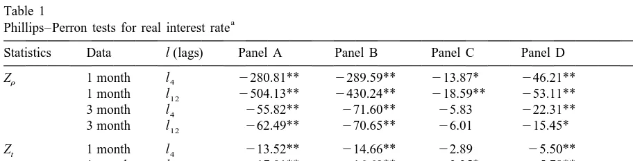
Following the methodology of Baillie and Bollerslev (1994) and Baillie et al. (1996), we conduct the Phillips–Perron unit root tests to study whether the ex post real interest rate is an I(1) process since the Augmented Dickey–Fuller (ADF) tests have low power against long memory alternatives (Diebold and Rudebusch, 1991). Moreover, KPSS (Kwiatkowski et al., 1992) tests are performed to test whether the ex post real interest rate is truly an I(0) process against long memory alternatives (including I(1) as a special case, see Lee and Schmidt, 1996). If both the null hypotheses of the Phillips–Perron tests and the KPSS tests are rejected, then the data series could be a long memory process. Before presenting our testing results, we note that both Phillips–Perron unit root test and KPSS test need to specify the lag length in the semiparametric estimation of the long run variance of the regression residuals. However, there is no well accepted rule to choose the lag length. The basic rule is that the lag length must increase with the sample size (Newey and West, 1987). We use the criteria of Schwert (1989) in this paper which has been popularly used in the literature. Furthermore, Bartlett windows (triangular windows) are used to ensure the non-negativity of the estimate of the long run variance of the regression residuals.
Table 1 contains the results of the Phillips–Perron unit root tests on the ex post real interest rate. Since the data series do not have a significant trend, we only include the constant term and the lagged data series in the regressors. The null hypothesis that the data series possess a unit root is strongly rejected in all sample periods except the November 1979–October 1982 subperiod. The acceptance of a unit root in Panel C may be explained by the low power of the unit root tests when the sample size is small (sample size is 36).
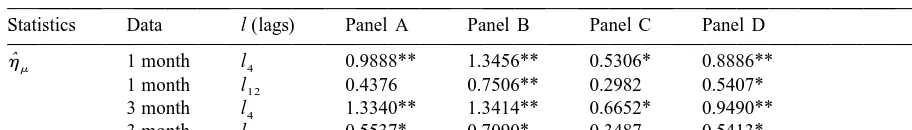
Table 2 displays the outcomes of the KPSS test on the ex post real interest rate. As mentioned
ˆ
above, we only employ the hm statistic which uses level stationary as its null hypothesis. The results
1 / 4
reveal that the null hypothesis is rejected in all sample periods when we use l45[4(T / 100) ] lag
Table 1
a
Phillips–Perron tests for real interest rate
Statistics Data l (lags) Panel A Panel B Panel C Panel D
Zr 1 month l4 2280.81** 2289.59** 213.87* 246.21**
1 month l12 2504.13** 2430.24** 218.59** 253.11**
3 month l4 255.82** 271.60** 25.83 222.31**
3 month l12 262.49** 270.65** 26.01 215.45*
Zt 1 month l4 213.52** 214.66** 22.89 25.50**
1 month l12 217.01** 216.60** 23.25* 25.78**
3 month l4 25.47** 26.36** 21.78 23.49*
3 month l12 25.77** 26.32** 21.81 22.96*
a
ˆ
Z , Phillips–Perron modified T(r 2r 1) statistic; Z , Phillips–Perron modified t statistic. *, significance at the 5% level;t
Table 2
a
KPSS test for real interest rate
Statistics Data l (lags) Panel A Panel B Panel C Panel D
ˆ
hm 1 month l4 0.9888** 1.3456** 0.5306* 0.8886**
1 month l12 0.4376 0.7506** 0.2982 0.5407* 3 month l4 1.3340** 1.3414** 0.6652* 0.9490** 3 month l12 0.5537* 0.7090* 0.3487 0.5413*
a
ˆ
hm, KPSS test with level stationary as the null hypothesis. *, significant at the 5% level; **, significant at the 1% level.
length, where [X] stands for the integer part of X, and T is the sample size. According to the simulation results of Lee and Schmidt (1996), we realize that the increase of the lag length to reduce the size distortion of the test statistic will decrease the power of the KPSS tests at the same time. This may explain why the null hypothesis is not rejected in the November 1979–October 1982 subperiod when we use the l12 lag length. Combing the results of the unit root tests and those of the KPSS test, we doubt that the ex post real interest rate is either an I(1) or an I(0) process. Instead, it could be an
I(d ) process, that is an integrated process of order d, where 0,d,1; these have received a lot of
attention recently. The following section summarizes some basic characteristics of the I(d ) process.
3. Long memory process
A process Y is said to be AutoRegressive Fractionally Integrated Moving Average process of ordert
p, d, q, denoted as ARFIMA( p,d,q) or I(d ), if it is defined as:
d
f(L )(12L ) (Yt2m)5u(L )at
wherem is the population mean, L is the usual lag operator,f(L ) is a pth degree polynomial, d is the differencing parameter which can be a fractional number,u(L ) is a qth degree polynomial, the zeroes of f(L ) and u(L ) lie outside the unit circle, f(L ) and u(L ) have no common zeroes, and the
2
innovation sequence a is a white noise with zero mean and variancet sa. The fractional differencing
d d ` j
operator (12L ) has the following binomial expansion: (12L ) 5oj50cjL , wherecj5G( j2d ) /
G( j11)G(2d ), and G(?) is the gamma function.
For the fractional white noise process, it is defined as:
d
(12L ) Yt5at
which is the simplest case of the ARFIMA model. This process is first introduced by Granger (1980, 1981), Granger and Joyeux (1980), and Hosking (1981). They show that Y is stationary when dt ,0.5 and is invertible when d. 20.5. Please refer to Baillie (1996) for the details.
Table 3
2 d 2 a
Estimation of monthly real interest rate (12f1L2f2L )(12L ) (Yt2m)5(11u1L1u2L )et
Estimates Panel A Panel B Panel C Panel D
d 0.666 (3.665) 0.204 (5.176) 0.275 (1.557) 0.193 (1.799)
f1 0.429 (3.315) – – –
f2 – – – –
m 1.420 (1.208) 0.540 (1.364) 3.230 (1.905) 3.355 (4.307) u1 20.797 (29.758) – 0.345 (1.917) 0.326 (2.635)
u2 – – – –
2
s 6.724 (15.100) 5.860 (12.689) 11.282 (4.243) 6.490 (7.000)
Q(10) 7.982 14.970 7.815 10.623
a
t ratios for the coefficients are in parentheses.
Maximum Likelihood Estimator (MLE) under quite general conditional homoskedastic distributions. A description of the properties of the CSS estimator and its finite sample performance is presented in Chung and Baillie (1993).
4. Estimation of the real interest rate
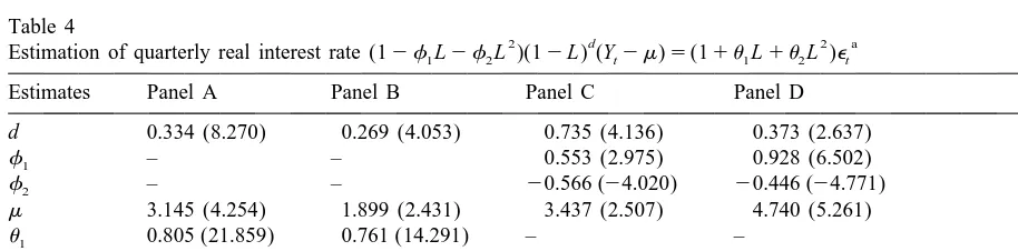
In this section, the CSS estimation of the ARFIMA model is applied to Mishkin’s data set. For each data series, ARFIMA( p,d,q) models are fitted, where p, q50, 1, 2. That is, there are nine combinations of the ARFIMA models fitted to each data series. The model selection criteria is based on the significance of the parameter estimates and the likelihood function. Of course, the portmanteau test is also considered. As is evident in Tables 3 and 4, the portmanteau test for remaining serial correlation in the residuals, Q(10), shows that the ARFIMA model provides a good description of temporal dependencies for the ex post real interest rate. For example, the best fitted model for the monthly real interest rate when we use the whole data set (Panel A) is ARFIMA(1,0.666,1). The results in Tables 3 and 4 indicate that the ex post real interest rate is mean reverting because all the differencing parameters are less than 1.
The results of Tables 3 and 4 also reveal that the estimate of the differencing parameter is larger when we use one quarter data in all subperiods. This phenomenon is compatible with the results of the
Table 4
2 d 2 a
Estimation of quarterly real interest rate (12f1L2f2L )(12L ) (Yt2m)5(11u1L1u2L )et
Estimates Panel A Panel B Panel C Panel D
d 0.334 (8.270) 0.269 (4.053) 0.735 (4.136) 0.373 (2.637)
f1 – – 0.553 (2.975) 0.928 (6.502)
f2 – – 20.566 (24.020) 20.446 (24.771) m 3.145 (4.254) 1.899 (2.431) 3.437 (2.507) 4.740 (5.261)
u1 0.805 (21.859) 0.761 (14.291) – –
u2 0.694 (18.080) 0.667 (16.170) – –
2
s 1.231 (15.100) 0.997 (12.689) 2.613 (4.243) 1.246 (7.000)
Q(10) 6.493 11.403 5.807 12.402
a
unit root tests conducted in this paper. For example, the estimate of the differencing parameter is 0.275 (not significantly different from 0) when we use one month data for the November 1979– October 1982 sample period and the null hypothesis of a unit root in the data series is rejected at the same time. Furthermore, the estimate of the differencing parameter is 0.735 when we use one quarter data for the same sample period and the results of the unit root tests are reversed. Therefore, the results of estimation provide us with further evidence of the correctness of the unit root tests performed in this paper.
5. Conclusions
This paper reexamines the time series properties of the US ex post real interest rate. The results of the Phillips–Perron unit root tests and the KPSS test indicate that the ex post real interest rate is neither an I(1) nor an I(0) process. Furthermore, the estimation of the ARFIMA model using the Conditional Sum of Squares (CSS) method reveals that the ex post real interest could be well described by an ARFIMA model with long memory. The persistence in the ex post real interest rate is larger than we thought before.
Acknowledgements
This research is supported by a grant from NSC 87-2415-H-260-004 of Taiwan. I would like to thank Professor Ching-Fan Chung for contributing the GAUSS program used to estimate the ARFIMA models.
References
Baillie, R.T., 1996. Long memory processes and fractional integration in econometrics. Journal of Econometrics 73, 5–59. Baillie, R.T., Bollerslev, T., 1994. Long memory in the forward premium. Journal of International Money and Finance 13,
565–571.
Baillie, R.T., Chung, C.-F., Tieslau, M.A., 1996. Analyzing inflation by the fractionally integrated ARFIMA-GARCH model. Journal of Applied Econometrics 11, 23–40.
Chung, C.-F., Baillie, R.T., 1993. Small sample bias in conditional sum-of-squares estimators of fractionally ARMA models. Empirical Economics 45, 293–297.
Clarida, R.H., Friedman, B.M., 1984. The behavior of US short term interest rates since October 1979. Journal of Finance 39, 671–682.
Diebold, F.X., Rudebusch, G.D., 1991. On the power of Dickey–Fuller tests. Economics Letters 35, 155–160. Fama, E.F., 1975. Short term interest rates as predictors of inflation. American Economic Review 65, 269–282.
Fama, E.F., Gibbons, M.R., 1982. Inflation, real returns and capital investment. Journal of Monetary Economics 9, 297–324. Granger, C.W.J., 1980. Long memory relationships and the aggregation of dynamic models. Journal of Econometrics 14,
227–238.
Granger, C.W.J., 1981. Some properties of time series data and their use in econometric model specification. Journal of Econometrics 16, 121–130.
Granger, C.W.J., Joyeux, R., 1980. An introduction to long-memory time series models and fractionally differencing. Journal of Time Series Analysis 1, 15–29.
Huizinga, J., Mishkin, F.S., 1984. Inflation and real interest rates on assets with different risk characteristics. Journal of Finance 39, 699–712.
Huizinga, J., Mishkin, F.S., 1986. Monetary policy regime shifts and the unusual behavior of real interest rates. Carnegie-Rochester Conference Series on Public Policy 24, 231–274.
Kwiatkowski, D., Phillips, P.C.B., Schmidt, P., Shin, Y., 1992. Testing the null hypothesis of stationarity against the alternative of a unit root: How sure are we that economic time series have a unit root? Journal of Econometrics 54, 159–178.
Lee, D., Schmidt, P., 1996. On the power of the KPSS test of stationarity against fractionally-integrated alternatives. Journal of Econometrics 73, 285–302.
Mishkin, F.S., 1981. The real rate of interest: An empirical investigation, the cost and consequences of inflation. Carneigie-Rochester Conference Series on Public Policy 15, 151–200.
Mishkin, F.S., 1988. Understanding real interest rates. American Journal of Agricultural Economics 70, 1064–1072. Mishkin, F.S., 1990. What does the term structure of interest rates tell us about future inflation? Journal of Monetary
Economics 25, 77–95.
Newey, W.K., West, K.D., 1987. A simple, positive semi-definite, heteroskedasticity and autocorrelation consistent covariance matrix. Econometrica 55, 703–708.
Roley, V.V., 1986, The response of interest rates to money announcement under alternative operating procedures and reserve retirement system, Working Paper No. 1812, National Bureau of Economic Research, Cambridge, MA.