www.elsevier.nlrlocateraqua-online
An empirical Bayes procedure for adaptive
forecasting of shrimp yield
David G. Whiting
), H. Dennis Tolley, Gilbert W. Fellingham
Department of Statistics, Brigham Young UniÕersity, ProÕo, UT, 84602, USA
Accepted 9 July 1999
Abstract
In order to make decisions regarding when to harvest cultured shrimp, short-term forecasts of future growth must be compared with expected future costs and changes in the value of the shrimp harvested. As with most agricultural products, researchers and business professionals collect and maintain data on the various factors that influence growth. Though many general fixed relation-ships between, say salinity, temperature, time and turbidity are known, exactly how these affect a particular crop changes from year to year. Vitality of the stock, unmeasured characteristics of the pond, and other factors which vary over time have a significant affect on the yield of a harvest. Consequently, to make reasonable short-term forecasts, forecasting models must include both the general factors gathered from past experience and crop specific variations from these overall effects. This paper presents a method of obtaining such a forecasting equation using a general mixed model setup currently available in many computer packages. These general formulas are illustrated with a real life example. SAS code necessary to implement the analysis is also included. The paper concludes by presenting a general equation for short-term forecasts using the estimates obtained from a SAS analysis.q2000 Elsevier Science B.V. All rights reserved.
Keywords: Bayes procedure; Shrimp; Forecasting
1. Introduction
For a corporation involved in the commercial farming of freshwater or marine organisms, there are a number of variables affecting profitability which must regularly be taken into account. One of the more important factors in determining net income is the decision of when to harvest the crop of organisms. If the company harvests too early,
)Corresponding author. Tel.:q1-801-378-4505; fax:q1-801-378-5722; E-mail: [email protected]
0044-8486r00r$ - see front matterq2000 Elsevier Science B.V. All rights reserved.
Ž .
it may be deprived of increased profit due to further growth. By harvesting too late, the corporation pays for additional feed and operating costs without realizing increased growth, thus reducing financial returns. Coupled with such considerations as market price at harvest, organism size, length of growing season, fertilizer or feed costs, and maintenance of capital equipment, it is important to be able to predict the yield for harvesting one or several weeks in the future.
In this paper, we illustrate a statistical approach for the adaptive forecasting of shrimp yield in the context of the following scenario. A shrimp farming corporation operates a series of 20 ostensibly identical 30-acre ponds in which the Pacific white shrimp
ŽPenaeus Õannamei is the sole species being grown. These ponds are traditionally.
harvested after a 22–27 week growth period, each period roughly corresponding to the
Ž .
dry and wet summer and winter, respectively seasons. The operators collect extensive data on each pond for each season and year including, but not limited to, daily measurements of morning and evening air and water temperature, daily measurements of salinity and water turbidity, and weekly measurements of average shrimp weight. Inasmuch as the variables influencing the growth of P.Õannamei have been addressed
Ž .
elsewhere see e.g., Bray et al., 1994; Wyban et al., 1995 , we will not specifically deal
Ž . Ž .
with them here. Likewise, Leung and Hochman 1990 ; Hochman et al. 1990 ; Leung et
Ž . Ž .
al. 1993 , and Tian et al. 1993 have considered shrimp farming in a broad economic
Ž . Ž .
framework. For instance, Hochman et al. 1990 and Leung and Hochman 1990 present a complete management model for determining the optimal stocking and harvesting schedules of farmed shrimp based on a series of decision rules. Rather than addressing all of the issues pertaining to such a management model, we focus exclu-sively on the methodology needed to compute an adaptive forecast given data from previous years and year-to-date data for the current year. This component could then easily be included in the growth estimation portion of the economic model provided by
Ž . Ž .
either Hochman et al. 1990 or Leung and Hochman 1990 .
Prediction of future growth entails two components. First, a regression equation is typically used to model the average growth rate of the organism over time. Subse-quently, the individual characteristics of the current crop of organisms which cause their growth rate to differ from previous crops are also accounted for in the model. These include such things as weather and environmental conditions peculiar to the current year, the viability of the original stock, and so forth. As the crop matures, the importance of these characteristics becomes more evident and therefore should be used in conjunction with modeled averages to predict growth. Thus, the problem is how to use past years’ information adjusted for current conditions to determine the optimal harvest time during the current year.
Ž .
The approach requires the following steps: 1 the assessment of which measured
Ž .
variables are significant predictors of growth, 2 the estimation of variability across
Ž .
ponds, years, and seasons, 3 the calculation of a random coefficients growth curve
Ž .
model for the historical data, and 4 the use of conditional probability to give adaptive forecasts of shrimp yield. In statistical nomenclature, this is referred to as either an
Ž .
empirical Bayes procedure Carlin and Louis, 1996 or, in traditional statistical terms, as
Ž .
2. Growth curve models
Ž .
Wishart 1938 was the first to consider the problem of analyzing growth rates. These models, known as random coefficient models in the statistical literature, have since
Ž
received considerable attention see, for example, Rao, 1959; Potthoff and Roy, 1964;
.
Grizzle and Allen, 1969; Laird and Ware, 1982; or Littell et al., 1996, chapter . Suppose we measure the total mass of shrimp in each pond on a weekly basis for a given year and season, say summer 1995. Conceptually, ‘‘pond’’ is the experimental unit whose growth we measure over time. Let us assume that shrimp growth rates for summer 1995 are similar across ponds due to identical weather conditions, similar feed, turbidity, salinity, and so on. A simple linear model to describe this average growth is
yi jsb0qb1wi jqb2wi j2q´i j
Ž .
1 where y is the yield, w is the week number, w2 is the week squared, and ´ is thei j i j i j i j
error associated with the ith pond and jth week. The reason for including the square of the weeks is to account for a nonlinear growth rate over time. Explicitly, when the initial rate of growth is nearly linear but tapers off as the shrimp get closer to full size, the growth curve flattens out. The square term in the model provides for this.
Ž .
The 20 ponds can be thought of as a random sample from a hypothetical population
Ž .
of summer 1995 ponds represented by Eq. 1 . Define the growth curve equation for a specific pond i as
y sb qb w qb w2qe
Ž .
2i j 0 i 1 i i j 2 i i j i j
where e are assumed to be Gaussian errors with mean zero and variance s2. The i j
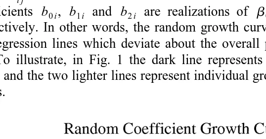
coefficients b , b0 i 1 i and b2 i are realizations of b0, b1 and b2 for the ith pond,
Ž .
respectively. In other words, the random growth curves for each pond given in Eq. 2 are regression lines which deviate about the overall population growth curve given by
Ž .1 . To illustrate, in Fig. 1 the dark line represents a hypothetical population growth curve and the two lighter lines represent individual growth curves from two hypothetical ponds.
Ž . Ž .
From Eq. 2 , we see that the error term ´i j for the overall linear growth model 1 consists of deviations from the population parameters plus random error, i.e.,
´i js
Ž
b0 iyb0.
qŽ
b1 iyb1.
wi jqŽ
b2 iyb2.
wi j2qe .i jŽ .
We can rewrite the growth curve Eq. 1 as
yi jsb0qb1wi jqb2wi j2q
Ž
b0 iyb0.
qŽ
b1 iyb1.
wi jqŽ
b2 iyb2.
wi j2qe .i jFor purposes of prediction, the b coefficients and s2
are estimated from previous years’ data. The b coefficients, however, are peculiar to the specific pond, season and year.
Ž .
To further refine the model in Eq. 1 for the ith pond and jth week, we add terms for the covariates temperature, t , salinity, s , and turbidity, u . The new model isi j i j i j
yi jsb0qb1wi jqb2wi j2qb3 i jt qb4si jqb5ui jqb6 i jt wi j
qb s w qb u w qb t w2qb s w2qb u w2q´ .
Ž .
37 i j i j 8 i j i j 9 i j i j 10 i j i j 8 i j i j i j
Here b0 is the coefficient for the y-intercept,b1 is the coefficient for linear growth in weeks and b2 is the coefficient for growth in squared weeks. The coefficients for temperature, salinity and turbidity are given by b3, b4 and b5, respectively. The remaining coefficients,b6 throughb11, are for various interactions of interest. Note that
Ž .
further interactions e.g., b12 i j i jt s wi j could have been included in this model.
Ž .
It is illustrative to write Eq. 3 as
yi js
Ž
b0qb3 i jt qb4si jqb5ui j.
qŽ
b1qb6 i jt qb7 i js qb8ui j.
wi jq
Ž
b qb t qb s qb u.
w2q´ .Ž .
42 9 i j 10 i j 11 i j i j i j
Hereb0, b3,b4 and b5 are the coefficients for the intercept of the growth curve, b1,
b6, b7 and b8 are the coefficients for the linear slope of the curve, and b2, b9,b10 and
b11 are the coefficients for the quadratic portion of the model. More specifically, for example, b7 and b10 measure the effect of salinity on linear and quadratic growth, respectively.
In certain situations it may be reasonable to assume a no-intercept model, in which
Ž .
estimate adjustments to the historical growth curve coefficients. These corrected coeffi-cients can then be used to forecast growth in the current year.
3. Random coefficient growth curve analysis
The analyses presented here were carried out using the Mixed procedure from the
Ž
statistical software package SAS. Instructions for the SAS package can be found in SAS
.
Language Reference Manual, Version 6, SAS Institute Note that SAS’s Proc Mixed is a
very powerful procedure for analyzing many types of mixed linear models, random coefficient growth curves being only one. For more details on mixed models, see e.g.,
Ž . Ž . Ž .
Scheffe 1959 ; Searle et al. 1992 , or Christensen 1987 . Additionally, see Littell et al.
Ž1996 for a thorough discussion and some excellent examples of mixed model analysis.
in SAS.
3.1. Preliminary analysis
An initial investigation of the data entailed creating a growth curve model for all 4 years and both seasons. The purpose of such a preliminary analysis is to decide on an appropriate model upon which later prediction will be based. Our model was refined as follows.
Ž . Ž .
After comparing results from using the general Eq. 4 and the no-intercept Eq. 5 , the no-intercept model was deemed most appropriate for modeling shrimp growth. The reasons for this are two-fold. First, the operators did not measure yield until 5 or 6
Ž
weeks after shrimp were introduced into the ponds i.e., when the shrimp were large
.
enough to be captured by the nets being used for measurement . Thus, information on these first few weeks of growth was unavailable and, in practical terms, yield could be considered to be zero at week 0. Secondly, since our goal is prediction at the upper end of the growth curve, the growth behavior at this low end of the curve had very little influence on the forecasts of interest. In other words, using the no-intercept constraint did not significantly alter our prediction results.
This preliminary analysis also showed that growth rates for individual ponds were not necessarily similar from year to year. Furthermore, the variability found within growth periods was not uniform. For instance, the growth curves for a set of ponds in summer 1994 were markedly more variable than the growth curves for the same set of ponds in summer 1996.
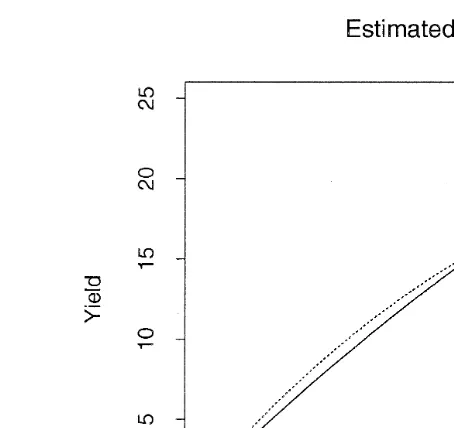
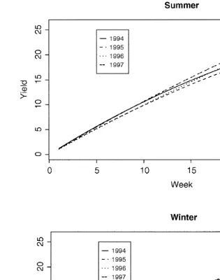
Most importantly, growth rates were shown to be consistent within seasons across different years but not between seasons within the same or different years. In short, summer growth rates differed significantly from winter growth rates. As shown in Fig. 2, although winter growth has a faster linear increase than summer, the growth rate also flattens out earlier. Fig. 3 shows the estimated growth curves for each year for the summer and winter seasons. Note that the variability of growth rates within a season between years is small compared with the variability between seasons.
Fig. 2. Overall estimates of summer and winter shrimp growth.
predictors in summer, salinity and turbidity were significant winter growth predictors. Since the predictive factors were not the same for summer and winter, a separate growth rate model was constructed for each season.
Stating that a factor is not statistically significant does not imply that it is unimportant in growth. For instance, the operators of the shrimp farm felt that turbidity was influential primarily in the first few weeks of growth. However, at least for the summer season, growth for that period may have been adequately described by other factors already in the model. In other words, if turbidity is highly correlated with one or more factors currently in the model, its inclusion is not necessary for purposes of prediction. The exclusion of temperature in winter illustrates another reason a factor which has an obvious impact on growth may be found insignificant. Specifically, if the factor shows little variation over the growth period, its role in prediction may be minimal. In the winter seasons, temperature levels fluctuated very little over time with an observed standard deviation of only 1.48C, hence its exclusion is not surprising. Thus, a factor may be statistically insignificant in the growth curve model although its impact on growth is unquestioned.
3.2. Summer growth curÕe analysis
Fig. 3. Estimated growth rates for 1994–1997.
of growth. Since a no-intercept model was chosen for both summer and winter seasons,
Ž .
the model equation for summer is identical to Eq. 5 except that b8 and b11, the coefficients for the effect of turbidity on linear and quadratic growth, respectively, are omitted. The summer model is thus
y s
Ž
b qb t qb s.
w qŽ
b qb t qb s.
w2q´ .Ž .
6Assuming yield data starts at week one and lasts until week n, the matrix form of the
The three components of the historical data necessary for adaptive forecasting are 1
Ž . Ž .
the vector of coefficients b, 2 the covariance matrix of b denoted C and 3 the
2
ˆ ˆ
2overall variance s . We label the estimates of these three quantities b,C and s
ˆ
, respectively.Note that the b vector obtained from SAS includes coefficients for each year, i.e.,
X U
b s
Ž
b1Ž1 994.,b1Ž1995.,b1Ž1996.,b1Ž1997., . . . ,b10Ž1994.,b10Ž1995.,b10Ž1996.,b10Ž1997..
.Ž .
The six SAS ESTIMATE statements yield the estimates of b given in Eq. 7 averaged over all 4 years. Likewise, the covariance matrix of bU
output by the SAS command COVB is a 24=24 matrix. The estimates ofC may be calculated by using the matrix equationCsACU
AX whereCU
is the covariance matrix of bU
output by SAS and
withmdenoting the Kronecker product operator.
Ž
respectively. Note also that the lower diagonal portion of the matrix has been omitted as
.
it is symmetric.
4. Empirical Bayes analysis
The philosophy underlying empirical Bayes analysis is to combine data from previous years with current, year-to-date data in producing forecasts which reflect the overall form of historical patterns but are adapted for current conditions.
ˆ ˆ
2Recall that b,C and s
ˆ
are the historical components used in forecasting. Suppose we have collected 8 weeks of data for a particular pond in the current year. OrganizingŽ .
be a column vector containing weight measurements and a matrix of independent variables, respectively. To forecast weight for a future week, say week 10, we construct a row vector xX0 by entering values for that week in the same order as the values in the rows of X . Thus,0
xX0s
Ž
10,10 t ,10 s,100,100 t ,100 s ..
Since temperature and salinity are unknown for the week we are predicting, we can either enter average values based on the past few weeks or enter an outside forecasted value. For example, if a cold front is expected, one could place the forecasted temperature value into t. Additionally, if our interest is to predict for a specific pond, we
ˆ
ˆ
may use the pond-adjusted values of b. Note that the covariance matrix C would remain the same.
The matrix equation used to perform an empirical Bayes forecast of shrimp yield is given by
where Y is the forecasted yield and I is an identity matrix of appropriate dimension. In0
the context of this problem, the empirical Bayes estimator is identical to the estimated
Ž . Ž
best linear unbiased predictor BLUP from linear model theory. See Christensen, 1987
Ž .
for the derivation of Eq. 8 and Maritz and Lwin, 1989 or Carlin and Louis, 1996 for
.
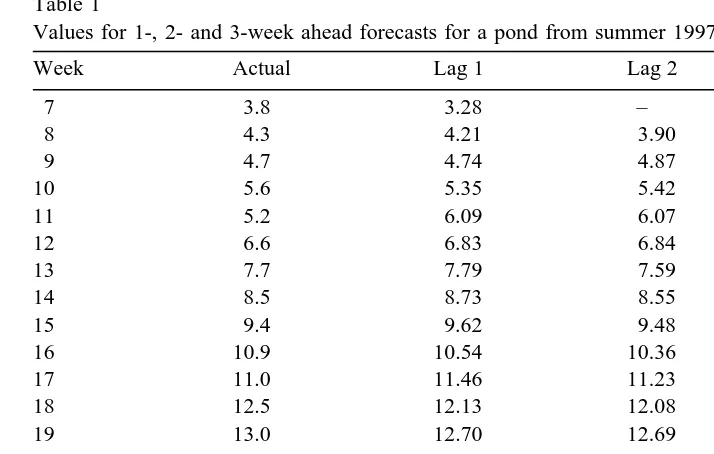
Table 1
Values for 1-, 2- and 3-week ahead forecasts for a pond from summer 1997
Week Actual Lag 1 Lag 2 Lag 3
7 3.8 3.28 – –
8 4.3 4.21 3.90 –
9 4.7 4.74 4.87 4.56
10 5.6 5.35 5.42 5.56
11 5.2 6.09 6.07 6.12
12 6.6 6.83 6.84 6.82
13 7.7 7.79 7.59 7.62
14 8.5 8.73 8.55 8.38
15 9.4 9.62 9.48 9.33
16 10.9 10.54 10.36 10.24
17 11.0 11.46 11.23 11.10
18 12.5 12.13 12.08 11.92
19 13.0 12.70 12.69 12.70
20 13.6 13.53 13.33 13.25
21 14.3 14.66 14.30 13.97
22 14.6 15.68 15.52 15.08
23 15.4 16.25 16.61 16.39
24 16.2 16.30 17.16 17.55
25 17.0 16.59 17.03 18.09
26 16.9 16.74 17.20 17.76
27 16.8 17.32 17.25 17.80
Ž . Ž .
In summary, the empirical Bayes Eq. 8 has the following components: 1 historical
ˆ ˆ
2 Ž .data gives us values for b,C and s
ˆ
, 2 year-to-date data gives us values for y and0Ž . X
X and 3 x is created by plugging in the week number as well as average or predicted0 0
values for the covariates temperature and salinity.
5. Forecasting example
We present as an example the forecasted growth curves for an individual pond from the summer of 1997. For lag-one forecasting, data from weeks 1–6 were used to predict week 7, then weeks 1–7 were used to predict week 8, and so on. Forecasts were computed at lags of 1, 2, and 3 weeks. Temperature and salinity values for the weeks being predicted were obtained by averaging the respective values from the two previous weeks. Table 1 shows the actual values plus the 1-, 2-, and 3-week ahead forecasts for this pond. Fig. 4 displays these data graphically.
From Fig. 4, note that the lag 1, lag 2, and lag 3 forecasts all follow the shape of the growth curve quite well. Although the lag 2 and lag 3 forecasts give slightly higher predictions of shrimp yield than were actually observed in the last few weeks of growth, they both do a remarkable job of predicting the point on the curve at which growth ceased and the curve flattened out. All other economic factors being equal, the optimal harvest time for this particular pond is week 25, a fact predicted at least three weeks earlier.
6. Conclusions
We have illustrated how the empirical Bayes method can be used to incorporate both historical data and data obtained on the current crop to make short-term predictions. This entailed estimating the overall growth curve as a function of weeks, salinity, temperature and turbidity. Analyses were done using the Proc Mixed procedure in SAS. Data on the current crop is also included in the empirical Bayes setup so that deviations of the current year from previous years can be included in the predictions. The example provided illustrated the ability of the prediction method to forecast 2 or 3 weeks into the future a downturn in the overall rate of growth. Using this in conjunction with other economic factors allows decision makers to estimate profit from harvest before the decision to harvest must be made.
The concept of adjusting estimates based on recent data epitomizes some of the advantages of Bayesian and empirical Bayesian methods. In the past, however, computa-tional demands made implementation of methods such as the shrimp example impracti-cal. Now that the computational difficulties have been reduced, the major reason for not using these methods appears to be a lack of understanding regarding their existence and ease of application. As illustrated here, the analysis to implement these procedures is not far removed from the common analysis of covariance approach. The results of the analysis can then be used to construct a prediction equation using matrix methods. This prediction equation constantly updates itself according to the most recent data available.
Acknowledgements
Appendix A. SAS code
DATA shrimp;
INFILE ‘shrimp.dat’;
INPUT pond year weeks weight temp turb sal; week2sweeks)weeks;
RUN;
r)Summer Random Coefficients Growth Curve Model)r
PROC MIXED;
RANDOM weeks week2rTYPEsUN SUBJECTspond SOLUTION; ESTIMATE ‘weeks’ weeks)year 0.25 0.25 0.25 0.25;
ESTIMATE ‘temp)weeks’ temp)weeks)year 0.25 0.25 0.25 0.25; ESTIMATE ‘sal)weeks’ sal)weeks)year 0.25 0.25 0.25 0.25; ESTIMATE ‘week2’ week2)year 0.25 0.25 0.25 0.25;
ESTIMATE ‘temp)week2’ temp)week2)year 0.25 0.25 0.25 0.25; ESTIMATE ‘sal)week2’ sal)week2)year 0.25 0.25 0.25 0.25;
MAKE ‘COVB’ OUTssummer; RUN;
r)Create Covariance Matrix for Summer )r
PROC IML;
namess ‘weeks’,‘temp)weeks’,‘sal)weeks’,
4
‘week2’,‘temp)week2’,‘sal)week2’ ;
Ž .
print summer labels‘‘Summer Covariance Matrix’’
x
rownamesnames colnamesnames ;
Ž Ž ..
sessqrt diag summer ;
w
print se labels‘‘Standard Errors’’
x
rownamesnames colnamesnames ; RUN;
Appendix B
Parameter Estimate Std Error DF t
weeks y2.80645053 0.21371564 2073 y13.13
temp)weeks 0.09787990 0.00693497 2073 14.11
sal)weeks 0.01696653 0.00349486 2073 4.85
week2 0.17237805 0.01115053 2073 15.46
temp)week2 y0.00476407 0.00036008 2073 y13.23
sal)week2 y0.00082625 0.00017068 2073 y4.84
Ž . Ž .
Summer weeks temp)week2 temp)weeks sal)week2 sal)weeks week2
Ž . Ž .
weeks 0.0456744 0.0000656 y0.001339 7.2432ey6 y0.000132 y0.002227
Ž . Ž .
temp)weeks y0.001339 "2.36ey6 0.0000481 2.1237ey7 y5.335ey6 0.0000668
Ž . Ž .
sal)weeks y0.000132 2.5812ey7 y5.335ey6 y5.733ey7 0.0000122 5.8817ey6
Ž . Ž .
week2 y0.002227 y3.714ey6 0.0000668 y3.99ey7 5.8817ey6 0.0001243
Ž . Ž .
temp)week2 0.0000656 1.2966ey7 y2.36ey6 y9.545ey9 2.5812ey7 y3.714ey6
Ž . Ž .
sal)week2 7.2432ey6 y9.545ey9 2.1237ey7 2.9133ey8 y5.733ey7 y3.99ey7
References
Bray, W.A., Lawrence, A.L., Trujillo, J.R., 1994. The effect of salinity on growth and survival of Penaeus
Õannamei, with observations on the interaction of IHHN virus and salinity. Aquaculture 122, 133–146.
Carlin, B.P., Louis, T.A., 1996. Bayes and Empirical Bayes Methods for Data Analysis. Chapman and Hall, London.
Christensen, R., 1987. Plane Answers to Complex Questions: The Theory of Linear Models. Springer-Verlag, New York.
Grizzle, J.E., Allen, D.M., 1969. Analysis of growth and dose response curves. Biometrics 25, 357–381. Hochman, E., Leung, P.S., Rowland, L.W., Wyban, J.A., 1990. Optimal scheduling in shrimp mariculture: A
stochastic growing inventory problem. American Journal of Agricultural Economics 72, 382–393. Laird, N.M., Ware, J.H., 1982. Random-effects models for longitudinal data. Biometrics 38, 963–974. Leung, P.S., Hochman, E., 1990. Modeling shrimp production and harvesting schedules. Agricultural Systems
32, 233–249.
Leung, P.S., Lee, D.J., Hochman, E., 1993. Bioeconomic modelling of shrimp and prawn: a methodological
Ž .
comparison. In: Kinnucan, H.W., Hatch, L.U. Eds. , Aquaculture: Methods and Economics, Chapter 3. Westview Press.
Littell, R.C., Milliken, G.A., Stroup W.W., Wolfinger, R.D., 1996. SAS System for Mixed Models. SAS Institute, Cary, NC.
Maritz, J.S., Lwin, T., 1989. Empirical Bayes Methods. Chapman and Hall, London.
Potthoff, R.F., Roy, S.N., 1964. A generalized multivariate analysis of variance model useful especially for growth curve problem. Biometrika 51, 313–326.
Scheffe, H., 1959. The Analysis of Variance. Wiley, New York.
Searle, S.R., Casella, G., McCulloch, C.E., 1992. Variance Components. Wiley, New York.
Tian, X., Leung, P.S., Hochman, E., 1993. Shrimp growth functions and their economic implications. Aquacultural Engineering 12, 81–96.
Wishart, J., 1938. Growth rate determination in nutrition studies with bacon pig and their analysis. Journal of the American Statistical Association 74, 215–221.
Wyban, J., Walsh, W.A., Godin, D.M., 1995. Temperature effects on growth, feeding rate and feed conversion
Ž .