Classification of Protein Sequences using the
Growing Self-Organizing Map
Norashikin Ahmad, Damminda Alahakoon, Rowena Chau
Clayton School of Information TechnologyMonash University Clayton, Victoria, Australia
Email: {norashikin.ahmad, damminda.alahakoon, rowena.chau}@infotech.monash.edu.au
Abstract— Protein sequence analysis is an important task in bioinformatics. The classification of protein sequences into groups is beneficial for further analysis of the structures and roles of a particular group of protein in biological process. It also allows an unknown or newly found sequence to be identified by comparing it with protein groups that have already been studied. In this paper, we present the use of Growing Self-Organizing Map (GSOM), an extended version of the Self-Organizing Map (SOM) in classifying protein sequences. With its dynamic structure, GSOM facilitates the discovery of knowledge in a more natural way. This study focuses on two aspects; analysis of the effect of spread factor parameter in the GSOM to the node growth and the identification of grouping and subgrouping under different level of abstractions by using the spread factor.
Keywords— protein sequence, classification, clustering, self-organizing map
I. INTRODUCTION
uman Genome Project [1] has resulted in a rapid increase of biological data including protein sequences in the biological databases. This situation has led to the need for effective computational tools that are essential for analyzing very large amount of data.
Being the product of molecular evolution, protein sequences provide a lot of information. Sequences which are highly similar have diverged from a common ancestor and they usually have similar structure and perform the same roles in biological processes. The fundamental methods used in sequence analysis to identify similarities between protein sequences are pair-wise sequence comparison for comparing two sequences and multiple sequence alignment. The earliest method developed for pair-wise comparison is dynamic programming algorithm by Needleman and Wunsch [2] (global alignment) and Smith and Waterman [3] (local alignment). Dynamic programming is computationally expensive and could cater only a small number of sequences. FASTA [4] and BLAST [5] algorithms which employ heuristic techniques have been developed to overcome this problem; they are faster, but are less accurate than dynamic programming methods. On the other hand, the multiple
sequence alignment method is used to identify conserved motifs by aligning together a set of related or homologous sequences. From this alignment, a consensus pattern that characterizes a protein group or family can be discovered. This method has been utilized as a basis in classifying protein sequences into families in many secondary databases such as PROSITE [6] (uses regular expressions pattern) and Pfam [7] (uses Hidden Markov Models).
Classification of protein sequences into groups or families is beneficial as it enables further analysis to be made within a group. Identification of a new sequence such as its possible structure and function also can be made easier by comparing it with existing groups which have already been studied. Artificial neural networks have been widely used in solving problems in many areas including protein sequence classification [8-12]. The unsupervised neural networks such as Self-Organizing Map (SOM) [13] has some advantages over the supervised methods as it does not require examples in its learning process. SOM also can construct a non-linear projection of complex and high-dimensional input signal into a low dimensional map which at the same time provides the visualization of the cluster grouping. These properties have made SOM a very useful tool in biological data analysis and discovery.
as well as cluster relationship between protein sequence data
also has been analyzed.
In the following section, related works in protein sequence classification using neural networks has been described. The GSOM algorithm is explained in detail in Section III. Experimental results are presented and discussed in Section IV followed by the conclusion and future works in Section V.
II. PROTEIN SEQUENCE CLASSIFICATION USING NEURAL NETWORKS
Both supervised and unsupervised neural networks have been applied in protein classification task. Wu et al [11] has successfully developed a protein classification system based on feed-forward neural networks with back-propagation algorithm named ProCANS. This system consists of multiple neural networks modules with each module been trained for a particular protein sequence family. Although the system could classify the protein sequences with high accuracy, they require both input and output to be presented to the networks in the training session. Therefore, the protein family for each sequence and also the number of protein families must be known a priori.
Compared to supervised method, unsupervised neural networks such as Self-Organizing Map (SOM) can classify without knowledge about the output. SOM has been applied in protein sequence classification in [8-10, 18]. In [8], clustering of protein sequences has been carried out using map with different sizes. The effect of using different values of learning parameters to the final map also has been investigated. This work has been extended in [9], where other features of protein sequence also have been used to represent the input instead of using amino acid alphabets as in [8] . The study also includes the analysis for fast and slow learning protocol and comparison with conventional methods for biological sequence analysis. In another study [10], the capability of SOM as a tool to visualize the similarity between different types of protein sequences (domain sequences and segments of secondary structure) has been demonstrated. In [18], SOMs with different resolutions were generated and hierarchical structure was constructed by mapping the nodes at each consecutive resolution that contain the same sequences. By using this method, SOM can be used to discover taxonomic relationship between the protein groups such as family-subfamily relationship. From the literatures, it is evident that SOM is capable of identifying patterns from the protein sequences and classify them into their respective groups or families. Protein groups could also be easily identified as similar sequences have all been clustered together either in the same node or have been positioned at the adjacent nodes. Despite the advantages, similar to supervised method the number of output nodes in SOM still has to be determined in advance.
Other issues which have been addressed in the previous works are the feature extraction and encoding method for the protein sequences. Protein sequences are formed by combination of twenty amino acids, each represented by an alphabet. Every amino acid has its own characteristics or physicochemical properties that can influence structure
formation and function of the protein. Besides individual amino acid, researchers have also used these properties as features to maximize information extraction from the protein sequences. Examples of the physicochemical properties are exchange group, charge and polarity, hydrophobicity, mass, surface exposure and secondary structure propensity [19].
Before processing begins, the sequences features have to be encoded into input vectors that can be processed by the neural networks. There are two types of encoding method that have been used; direct [18] and indirect sequence encoding [9-11]. In the direct encoding, each amino acid is represented directly by its identity or its features by using binary numbers (0 and 1) as an indicator vector. For example, to represent an amino acid, we use 19 zeros with a single one in one of the positions to distinguish each amino acid type. Indirect sequence encoding involves the encoding of global information from the sequence as in residue frequency-based or n-gram hashing method, similar method used in natural language processing. Dipeptide frequency encoding or 2-gram has been applied in [8] and [9]. In [11] and [12], the application of various size of n-grams extraction with different amino acid features in classifying the protein sequences has been studied. Despite successful implementation of both encoding methods, they suffer from several limitations. Direct method requires sequences to be aligned first in order to get an equal length for all sequences. This method also gives a large number of input vectors due to the way sequence is encoded. Indirect method allows short sequence patterns or motifs which are significant for a protein function to be extracted. By using this method, pre-alignment of sequences is not required; however the position information may be lost.
III. GROWING SELF-ORGANIZING MAP (GSOM) GSOM has been developed as an improvement over SOM algorithm in clustering and knowledge discovery tasks. It has a dynamic structure whereby it starts with four initial nodes and grows node and connections as it is presented with data inputs. This ability allows the map to grow naturally reflecting the knowledge discovered from the data set in contrast to SOM, where the map structure is restricted to a predefined number of nodes. Spread factor (SF), a parameter introduced in the GSOM can be utilized in controlling the spread of the map. SF takes values from 0 to 1, with lower SF value for a lesser spread map and higher SF value for a larger spread map. The use of higher SF value results in finer clusters or subclusters being created. Therefore by using different SF values, maps with different resolutions can be generated and hierarchical analysis can be carried out.
The GSOM learning process includes three phases called initialization, growing and smoothing. In the initialization phase, weight vectors of the starting nodes are initialized with random numbers. The growth threshold (GT) for the given data set is then calculated by using this equation:
) ln(SF D
GT =− × (1)
In the growing phase, input is presented to the network and the winner node which has the closest weight vector to the input vector is determined using Euclidean distance. The weights of the winner and its surrounding nodes (in the neighborhood) are adapted as described by:
⎩
During the weight adaptation, learning rate used is reduced over iterations according to the total number of current nodes. The error values of the winner (the difference between the input vector and the weight vector) are accumulated and if the total error exceeds the growth threshold, new nodes will be grown if it is a boundary node. The weights for the new nodes are then initialized to match the neighboring nodes weights. For non-boundary nodes, errors are distributed to the neighbors. The growing phase is repeated for each input and can be terminated once the node growth has reduced to a minimum value.
The purpose of smoothing phase is to smooth out any quantization errors from the growing phase. There is no node growing in this phase; only weight adaptation process is carried out. A lesser value of learning rate is used and weight adaptation also is done in a smaller neighborhood.
IV. EXPERIMENTAL RESULTS
A. Data Preparation
Protein sequences used in the experiment were downloaded from the SWISS-PROT database (http://ca.expasy.org/sprot/). We have used three families of protein; cytochrome c, insulin and globin (with subfamilies of hemoglobin alpha chain (HBA) and hemoglobin beta chain (HBB)). Sample size of 100 sequences for each cytochrome c, insulin, HBA, and HBB group has been taken.
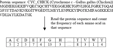
In this study, we have chosen frequency of single amino acid occurrence as the feature for the protein sequences. This method is also known as 1-gram extraction. We considered only 20 basic amino acids in the experiment (A, C, D, E, F, G, H, I, K, L, M, N, P, Q, R, S, T, V, W, and Y). Input vectors used in the network have 20 dimensions with each dimension represents the frequency of each amino acid in the sequences. After the feature extraction process was completed, the frequency values were scaled into values between zero and one. Example of the 1-gram extraction for a protein sequence (CYC_CHICK) is shown in the following figure.
Figure 1. Example of 1-gram extraction process in the experiment
The GSOM clustering process involves a setting of several parameters such as spread factor, R value, factor of distribution (FD) and learning rate. We used different values for the spread factor in each experiment to investigate its effect to the learning algorithm and final cluster formation. Learning rate value of 0.1, R value of 3.8 and FD value of 0.3 have been used throughout the experiment. For smoothing phase we set a smaller learning rate value of 0.05. In every experiment, GSOM was trained for 100 epochs with learning rate value reduced by half in each epoch.
B. Investigation on the Effect of Spread Factor to the Node Growth
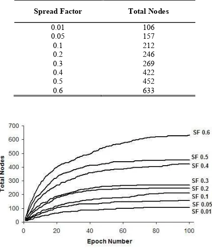
We have investigated the effect of the spread factor values to the growing phase of GSOM by recording the total number of nodes in each epoch. The total number of nodes generated for different SF values are shown in Table I. It can be seen from Table I, the number of nodes increased with the addition of spread factor values. The node growth in GSOM is actually attributed to the growth threshold (GT) value. In the GSOM algorithm, the new node will grow when the accumulated error value of a node exceeds the GT. It can be concluded from (1) that a low spread factor value will result in a high GT causing a lesser number of nodes grow, and a high spread factor value gives a low GT thus, allowing more nodes to be added.
The growing of nodes in every spread factor of the experiments is illustrated in Fig. 2. From the figure, we can see that as training progresses in each epoch cycle, GSOM continues adding more nodes to the map. However, the number of grown nodes is slowly decreased and then stabilized at a certain epoch cycle. The time (epoch cycle) when the nodes growth was reduced varied between spread factors. It can be observed that for all spread factors, the nodes growth has stabilized before reaching 100epoch cycles. This indicates that learning convergence in GSOM can be achieved in a small number of epoch cycles.
Protein sequence: CYC_CHICK (Cytochrome c - Gallus gallus (Chicken)) MGDIEKGKKIFVQKCSQCHTVEKGGKHKTGPNLHGLFGRKTGQAE GFSYTDANKNKGITWGEDTLMEYLENPKKYIPGTKMIFAGIKKKSER VDLIAYLKDATSK
Read the protein sequence and count the frequency of each amino acid in that sequence
TABLE I. SPREAD FACTOR AND TOTAL NODES
Spread Factor Total Nodes
0.01 106 0.05 157 0.1 212 0.2 246 0.3 269 0.4 422 0.5 452 0.6 633
Figure 2. Change to total number of nodes at each epoch cycle for various spread factor values
C. Identification of Grouping and Subgrouping in Protein Sequences under Different Level of Abstractions
The visualization of the clusters obtained from the clustering of the protein sequences using GSOM for spread
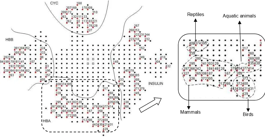
factor 0.01 and 0.5 are shown in Fig. 3 and Fig. 4 respectively. From the figures, white square nodes indicate the first four initial nodes whereas nodes labeled with numbers represent the hit nodes (winner nodes). It can be seen from both figures that GSOM has successfully identified patterns from the dataset and organized them such that sequences belong to the same group have been positioned in nodes that adjacent to each other. The four groups have also been clearly separated on the map with each group was positioned exclusively in its own region. Interestingly, GSOM could also differentiate the subgrouping of protein sequences within the same protein family. This can be observed from the map, in case of HBA and HBB groups in which both are belong to the same family (globin family). HBA and HBB groups have been placed next to each other in both maps indicating the close relationship between the two groups. Although in other lower spread factor maps (figures not shown) the boundary that separated these two groups sometimes was not clear, they remained in the same region and separated from the CYC and insulin families clusters.
From Fig. 3, we can see that GSOM could distinguish patterns from the four groups even at a very low spread factor. Further analysis into every node also showed that most of the nodes consist of sequences from the same family except for few nodes. This includes node 80, which contains nine insulin sequences and a HBB sequence (HBB_OREMO); node 12, which contains a HBA sequence (HBA_LEIXA) grouped with five HBB sequences and lastly node 3, which two HBB sequences (HBB_NOTAN and HBB_GYMAC) have been grouped with other nine HBA sequences. It is also interesting to point out that most of the sequences in these nodes are from aquatic animals. The incorrect classification happened probably because of the high similarity in the composition of the amino acid between the sequences of aquatic animals under study.
Figure 3. GSOM at SF 0.01 and example of subgroups identified from the map.
Aquatic animals Birds Mammal
Reptiles
Figure 4. GSOM at SF 0.5. The formation of subgroups for HBA sequences is shown on the right side of the figure.
Hemoglobin and CYC families have been used in phylogenetic analysis using self-organizing tree network (SOTA) in [20]. The selection of these families is because they evolve slowly compared to the others; therefore, the patterns are more conserved. In phylogenetic analysis, protein sequences can be grouped according to their species and the evolutionary relationship among the species can be inferred. The results obtained from the experiments with GSOM have shown that this algorithm is also capable of grouping the sequences according to their taxonomic groups. This can be observed from Fig. 3, for instance, node 37, 50, 51, 62, 68, 69 and 97 consist of mammals; node 17, 18 and 27 contain birds; and node 36 which comprise of reptiles. As can be seen from Fig. 3, the nodes that belong to the same animal group are located next to each other on the map. A subgroup of aquatic animals was found for nodes 23, 12, 3 and 13. This subgroup was actually formed by nodes which belong to separate protein groups; node 13 and 23 are from insulin group whereas node 12 and 3 are from HBA and HBB group. This finding suggests that there may be some similarities for amino acid compositions for aquatic animals even though the sequences are from different groups or families. Another significant result was found from insulin group, where sequences that belong to insulin-like growth factor I precursor protein and insulin-like growth factor II precursor protein (where ids start with IGF1 and IGF2 respectively) have been grouped separately from other insulin sequences (ids start with INS). In Fig. 3, the IGF1 and IGF2 sequences are populating node 93, 95, 83, 96, 91 and 66.
In Fig. 4, GSOM with SF 0.5 is presented. As shown in this figure, the four groups of CYC, insulin, HBA and HBB sequences can be identified easily as they have been spread out into four distinct directions. From Fig. 4, we can see that nodes
with zero hit can also be used to visualize the separation between groups. As the spread factor value used was higher, a larger number of nodes have been obtained. Further investigation revealed that more specific classification has occurred to the protein sequences. For CYC sequences in SF 0.01, all mammals, birds and reptiles have been clustered into the same node (node 48). However, in SF 0.5 some of these sequences have been split up into different nodes. Similar situation happened to the other three groups but HBA has the most number of nodes split among the others. In case of subgroup formation, nodes from HBA group have formed four subgroups, with each subgroup corresponds to an animal group. From the map, subgroups of nodes comprising sequences from mammals, reptiles, aquatic animals and birds have been discovered.
Interestingly, we found that some of the nodes in the subgroups contain specific type of animal. For example in HBA’s mammal’s subgroup, node 297 presents sequences from spider monkey, assam’s monkey, chimpanzee, gorilla, marmoset, and green monkey. Node 129 and 203 which are adjacently mapped contain sequences of lion, jaguar, tiger and leopard. Other examples are node 206 (red panda and giant panda), node 241 (Indian elephant and African elephant), node 272 (llama, alpaca, camel and guanaco) and node 205 (polar bear and black bear).
V. CONCLUSION
In this paper, we have shown that GSOM is capable of discovering knowledge in protein sequences. The results of the study indicate that GSOM can be used to classify protein sequences and identify the grouping as well as subgrouping from the protein sequences. Even though we have used only 1-gram extraction as the feature for the protein sequences,
Birds Mammals
GSOM could successfully classify the sequences into the
expected groups. By changing the spread factor value, the formation of groups under different level of abstractions can be achieved. Further research might investigate the effect of using different protein sequence encoding methods such as 2-gram on the protein classification using the GSOM. It would also be interesting to see the formation of the clusters as a result of using other protein sequence features such as exchange group and hydrophobicity in the classification.
REFERENCES
[1] "Human Genome Program," U.S. Department of Energy 1997.
[2] S. B. Needleman and C. D. Wunsch, "A general method applicable to the search for similarities in the amino acid sequence of two proteins,"
Journal of Molecular Biology, vol. 48, pp. 443-453, 1970.
[3] T. F. Smith and M. S. Waterman, "Comparison of biosequences,"
Advances in Applied Mathematics, vol. 2, pp. 482-489, 1981.
[4] D. J. Lipman and W. R. Pearson, "Rapid and Sensitive Protein Similarity Searches," Science, vol. 227, pp. 1435-1441, 1985.
[5] S. F. Altschul, W. Gish, W. Miller, E. W. Myers, and D. J. Lipman, "Basic local alignment search tool," Journal of Molecular Biology, vol. 215, pp. 403-410, 1990.
[6] N. Hulo, A. Bairoch, V. Bulliard, L. Cerutti, B. Cuche, E. De Castro, C. Lachaize, P. S. Langendijk-Genevaux, and C. J. A. Sigrist, "The 20 years of PROSITE," Nucleic Acids Res. 2008, vol. 36, January 2008. [7] R. D. Finn, J. Mistry, B. Schuster-Bockler, S. Griffiths-Jones, V.
Hollich, T. Lassmann, S. Moxon, M. Marshall, A. Khanna, R. Durbin, S. R. Eddy, E. L. L. Sonnhammer, and A. Bateman, "Pfam: clans, web tools and services," Nucleic Acids Res., vol. 34, pp. D247-251, January 1, 2006 2006.
[8] E. A. Ferran and P. Ferrara, "Topological maps of protein sequences,"
Biological Cybernetics, vol. 65, pp. 451-458, October, 1991 1991. [9] E. A. Ferran, B. Pflugfelder, and P. Ferrara, "Self-organized neural maps
of human protein sequences," Protein Science, vol. 3, pp. 507-521, March 1, 1994 1994.
[10] J. Hanke and J. G. Reich, "Kohonen map as a visualization tool for the analysis of protein sequences: multiple alignments, domains and segments of secondary structures," Comput. Appl. Biosci., vol. 12, pp. 447-454, December 1, 1996 1996.
[11] C. Wu, G. Whitson, J. McLarty, A. Ermongkonchai, and T. C. Chang, "Protein classification artificial neural system," Protein Science, vol. 1, pp. 667-677, May 1, 1992 1992.
[12] C. H. Wu, A. Ermongkonchai, and T.-C. Chang, "Protein classification using a neural network database system," in Proceedings of the Conference on Analysis of Neural Network Applications Fairfax, Virginia, United States: ACM, 1991.
[13] T. Kohonen, "The self-organizing map," Proceedings of the IEEE, vol. 78, pp. 1464-1480, 1990.
[14] D. Alahakoon, S. K. Halgamuge, and B. Srinivasan, "Dynamic self-organizing maps with controlled growth for knowledge discovery,"
IEEE Transactions on Neural Networks vol. 11, pp. 601-614, 2000. [15] A. L. Hsu, S.-L. Tang, and S. K. Halgamuge, "An unsupervised
hierarchical dynamic self-organizing approach to cancer class discovery and marker gene identification in microarray data," Bioinformatics, vol. 19, pp. 2131-2140, 2003.
[16] H. Wang, F. Azuaje, and N. Black, "An integrative and interactive framework for improving biomedical pattern discovery and visualization," IEEE Transactions on Information Technology in Biomedicine, vol. 8, pp. 16-27, 2004.
[17] C.-K. K. Chan, A. L. Hsu, S.-L. Tang, and S. K. Halgamuge, "Using Growing Self-Organising Maps to Improve the Binning Process in Environmental Whole-Genome Shotgun Sequencing," Journal of Biomedicine and Biotechnology, vol. 2008, p. 10, 2008.
[18] M. A. Andrade, G. Casari, C. Sander, and A. Valencia, "Classification of protein families and detection of the determinant residues with an improved self-organizing map," Biological Cybernetics, vol. 76, July, 1997 1997.
[19] C. H. Wu and J. W. McLarty, Neural networks and genome informatics. Amsterdam ; Oxford: Elsevier, 2000.
[20] H.-C. Wang, J. Dopazo, L. G. De La Fraga, Y.-P. Zhu, and J. M. Carazo, "Self-organizing tree-growing network for the classification of protein sequences," Protein Science, vol. 7, pp. 2613-2622, 1998.