Jurnal Teknologi, 48(D) Jun 2008: 113–141 © Universiti Teknologi Malaysia
MODELING AND CONTROLLER DESIGN FOR A COUPLED-TANK LIQUID LEVEL SYSTEM: ANALYSIS & COMPARISON
MOHD FUA’AD RAHMAT1 & SAHAZATI MD ROZALI2
Abstract. The system under investigation is a coupled-tank apparatus which is a laboratory bench top emulation of a common process in industrial control. The basic control principle of the coupled-tank system is to maintain a constant level of the liquid in the tank when there is an inflow and outflow of water in the tank and outflow of water out of the tank respectively. Classification of this system using system identification technique involved the transient response analysis, the pseudorandom binary sequence (PRBS) analysis and the least square method. The main objective of this project is to determine the mathematical model of a coupled-tank system using these techniques. It follows by designing a controller consists of a PID and a Fuzzy Logic controllers for the system. At the final stage of this project, the usage of both controllers in industrial applications is compared and analyzed.
Keywords: System identification, step response, pseudorandom binary sequence, least square method, PID & Fuzzy Logic controller
Abstrak. Sistem yang diuji ialah tangki berkembar yang biasa digunakan dalam proses kawalan industri. Prinsip asas sistem tangki berkembar adalah untuk mengekalkan paras cecair di dalam tangki pada suatu nilai tetap apabila wujud aliran keluar masuk cecair dalam tangki. Analisis tindak balas langkah, analisis pseudorandom binary sequence (PRBS) dan kaedah least square digunakan untuk mengklasifikasikan sistem ini. Objektif utama projek ini adalah untuk menentukan model matematik sistem tangki berkembar menggunakan tiga teknik tesebut. Ia diikuti dengan mereka bentuk pengawal yang terdiri daripada pengawal PID dan pengawal Fuzzy Logic untuk sistem ini. Pada peringkat akhir projek ini, penggunaan kedua-dua pengawal dalam aplikasi industri dibandingkan dan dianalisa.
Kata kunci: Pengenalpastian sistem, tindak balas langkah, pseudorandom binary sequence, kaedah
least square, pengawal Fuzzy Logic & PID
1.0 INTRODUCTION
The industrial application of liquid level control is tremendous especially in chemical process industries. Usually, the level control exists in some of the control loops of a process control system. Many other industrial applications are concerned with level
1 Department of Control and Instrumentation Engineering, Faculty of Electrical Engineering,
Universiti Teknologi Malaysia, 81310 Skudai, Johor Bahru, Malaysia
2 Department of Control, Instrumentation and Automation, Faculty of Electrical Engineering,
control, may it be a single loop level control or sometimes multi-loop level control. In some cases, level controls that are available in the industries are for interacting tanks.
Hence, level control is one of the control system variables which are very important in process industries. Mathematical modeling is a description of a system in terms of equations.
A system is often represented by a box called a black box as shown in Figure 1.
The system may have several inputs or excitations each of which is a function of time. Outputs are variables that are to be calculated or measured. There is a cause-and-effect relationship between the outputs and inputs. One approach to construct a mathematical model is to find equations that relate the outputs directly to the inputs by eliminating all the other variables that are internal to the system. System identification method is one of mathematical modeling method. It involves experimental modeling. Experiments and observations technique will be used to deduce model. However, this procedure needs prototype and real system.
1.1 System Identification
Identification is a determination on the basis of input and output of a system with a specified class of systems to which the system under test is equivalent whereas system is a collection of components which are coordinated together to perform a function. A model is needed in system identification technique. Model is a description of the system that should capture the essential information about the system. The principle used in this method is to estimate system from measurement of input, u(t) and output, y(t)[1].
Classification of the system using system identification technique involved nonparametric and parametric methods. Nonparametric methods that are used in this project consist of transient response analysis and correlation analysis[5]. Least square method is the parametric technique applied for this paper. A procedure of system identification technique occupied six stages. It starts with experimental design followed by data collection and data preprocessing. Next, a suitable model structure will be selected. Then, the important parameters of the model will be estimate. Finally, the model will be validated [2].
Figure 1 Black-box representation of a system
u2
un
u1
inputs outputs
y1
y2
1.2 Coupled-Tank CTS 001
Coupled-Tank CTS 001 is a computer-controlled coupled tank system that is used for liquid level control. It introduced a concept of virtual instrumentation[6]. This coupled tank uses LABWINDOWS/CVI development tools and National Instruments data acquisition card (NI-DAQ7) for data analysis, control and monitoring of the liquid level[8]. An IBM-PC is needed in order to control the operation of CTS 001. Figure 2 shows a diagram of Coupled-Tank CTS 001[3].
Figure 2 Overall diagram of Coupled-Tank CTS 001
1.3 Nonparametric Methods
Two nonparametric methods are selected to be applied in this project. Transient response analysis using step input as excitation force is used first followed by correlation analysis which used Pseudo Random Binary Sequence (PRBS) as input.
1.3.1 Transient Response Analysis
In transient response analysis, step input is injected to the system and the transfer function of the system can be obtained from the system output response. Since the transfer function is a representation of the system from input to output, the system’s step response can lead to a representation even though the inner construction is not known. With a step input, time constant and steady-state value can be measured from which the transfer function can be calculated.
Computer
1.3.2 Correlation Analysis
In correlation analysis, Pseudo Random Binary Sequence (PRBS) will be used as forcing functions for the system. Then the transfer function of the system can be obtained from the output correlation. There are two types of correlation functions:
(i) Auto-correlation function (ACF) (ii) Cross-correlation function (CCF)
The auto-correlation function of a signal x(t) is given as
( )
T( ) (
)
xx
T
T
x t x t dt T
ϕ τ τ
→∞ −
= lim 1
∫
+2 (1)
whereas the cross-correlation is defined as
( )
T( ) (
)
xx
T
T
x t y t dt T
ϕ τ τ
→∞ −
= lim 1
∫
+2 (2)
where ϕxx(τ) is the time average of the product of the function τ seconds apart as τ is allowed to vary from zero to some large value and the averaging being carried out over a long period 2T [1].
1.4 Parametric Method
The parametric method used in this project is Least Square Method.
1.4.1 Least Square Method
This technique provides us with a mathematical procedure by which a model can achieve a best fit to experimental data in the sense of minimum-error–squares. Least Square Method is the technique with a mathematical procedure by which a model can achieve a best fit to experimental data in the sense of minimum error squares. It is consistent, unbiased and efficient. The formulas used for this technique are:
1st order system: y k
( )
bz u k( )
az−
− =
−
1
1
1 (3)
2nd order system: y k
( )
(
b z b z)
u k( )
a z a z− −
− −
+ =
− −
1 2
1 2
1 2
1 2
1 (4)
1.5 Pseudorandom Binary Sequence (PRBS)
PRBS are probably the most convenient inputs for linear system identification. The ACF of a PRBS provides the best and useful approximations to periodic white noise. It is the forcing functions most widely used in statistical system testing. Their general form is shown in Figure 3.
Figure 3 General form of PRBS
There are two types of PRBS; Quadratic Residue Code (QRC) and Maximum Length Sequences (MLS). In this project, MLS is used as a forcing function of the system being identified. Length of MLS is given by
N = 2n – 1 (5)
where n is an integer.
This can be generated by an n stage shift register with the first stage determined by feedback of the appropriate modulo two sum of the last stage and one or two earlier stages. Figure 4 shows the generation of PRBS by shift register.
time period
+1
0
–1
Modulo two addition is the logic function “exclusive or”; if the inputs are different, the output is logic 1. The logic contents of the shift register are moved one stage to the right every ∆t seconds by simultaneous triggering by a clock pulse. All possible states of shift register are passed through except that of all zeros. The output of PRBS can be taken from any stage and is a serial sequence of logic states having cyclic period N ∆t. [1]
Figure 4 Generation of PRBS by shift register
Output Feedback
XOR
1.6 Controller
Controller is an equipment introduced to monitor a process and to adjust some variables in order to maintain the system at or near desired conditions. Two types of controller are selected to be applied in this project; the family of PID controller and Fuzzy Logic Controller. Then the usage of these two different controllers in industrial applications is compared.
1.6.1 PID Family Controller
PID family consists of Proportional controller, Proportional-Integral (PI) controller, Proportional-Derivative (PD) controller and Proportional-Integral-Derivative (PID) controller. These controllers is a type of feedback controller whose output, a control variable (CV) is based on the error between some user-defined set point (SP) and some measured process variable (PV). Each element of these controllers refers to a particular action taken on the error.
Proportional (P) only controller is used to increase magnitude response whereas Proportional-Integral (PI) controller will reduce a steady-state error. On the other hand, Proportional-Derivative (PD) controller will improve transient response of the system by reducing settling time; Ts. Proportional-Integrative-Derivative (PID) controller combines both all the advantages of each different controller to get a better response[4].
1.6.2 Fuzzy Logic Controller
Fuzzy Logic overcome the problems of crisp sets where instead of only true or false, yes or no, 1 or 0, a membership of degree from 0 to 1 can be assigned to a set. A fuzzy logic control system can be configured as shown in the block diagram in Figure 5.
Figure 5 Fuzzy Logic control system
Inference engine
Process Crisp control signal
Defuzzifier Fuzzy
Knowledge base
A fuzzy logic controller would normally take the readings of error (e) and the rate of change of error (∆e) as the inputs and the change in the control input (∆u) signal as its output. A fuzzifier then transforms the crisp values of e and ∆e into corresponding fuzzy values. From the knowledge or rule base, the fuzzy values of e and ∆e determine which particular rule or rules are to be fired through an inferencing algorithm. Several values of ∆u will then be obtained and a defuzzification mechanism will then transform these values into one crisp value. The actual control signal is obtained by adding ∆u to the past value of u which is sent to the plant. In this project, three groups of FLC are used where each group has 3 × 3 rules, 5 × 5 rules and 7 × 7 rules respectively. The response from each type is analyzed and compared between each other and PID family controllers [3].
2.0 EXPERIMENTAL SET-UP OF THE SYSTEM
Before using the coupled tank for the step response analysis, the tank should be calibrated first. The calibration process involved a level sensor calibration process for each tank and control inflow calibration process[7]. These processes have to be applied in order to ensure that the conversion between the actual measurements of the liquid level in cm to voltage is recorded by the software. This stage is followed by open loop analysis. In this analysis, firstly, step input is given to the system and from the response obtained, transfer function of the first-order and second-order system will be calculated. Then, pseudorandom binary sequence (PRBS) signal with 15 shift register in injected to the system. The input and output data of the tank is collected to plot autocorrelation graph. From the graph obtained, once again the transfer function of a first-order and second-order system is computed. The same data is used to acquire the transfer function of the system using least square method. The second stage is the closed-loop analysis where a suitable controller for each first-order and second-order system is designed. PID family controller is designed first using transient response tuning method followed by Fuzzy Logic controller design. Finally, the response of each system with two different controllers is compared and analyzed.
2.1 Results and Analysis
2.1.1 Calibration Process
Calibration process is important in order to understand the characteristics of the main components of the coupled tank control and to relate the theoretical aspects of the function of the components. Besides, the relationship between the system parameters and its effect on the system response can be observed through this process [3].
Basically, there are three important components of the apparatus that need serious studies and experimentation and these are:
(i) Tank dynamic characteristics (ii) Level sensor characteristics (iii) Pump characteristics
Calibration and measurement of the components characteristics are important to determine the relationship of the input and output of these components and also to determine whether there are non-linearities present which would explain some of the discrepancies in certain experimental results or any dead zones encountered in starting the flow of the pump.
The input to the pump motor is the voltage Ui acting as the actuated signal that control the input flow rate Qi to each tank. The liquid then goes into the tank and causes the level to rise to a certain height Hi. The level in the tank is measured using a sensor which consist of a capacitance probe and associated electronics.
The voltage Yi to level Hi relationship is quite linear and can be written as follows.
Yi = ksHi (6)
where ks = gain of level sensor (V/cm)
The value of ks is important to obtain the relationship between the height of liquid in the tank and the converted voltage corresponding to it. Figure 7 shows the relationship between the height of liquid in the tank A and the corresponding voltage.
Thus, from linearization, the gain of level sensor for Tank A
s
k = 0.177 V/cm
Figure 8 shows the relationship between the height of liquid in the tank B and the corresponding voltage.
Gain of level sensor for tank B, ks = 0.164 V/cm
The relationship of the pump flow rate Qi and the input voltage Ui is also linear. It can be written as equation (7).
Qi = kpUi (7)
where kp = gain of the pump (cm3/sec/V)
Figure 6 The block diagram of a single tank control system
Pump Tank sensorLevel
Voltage
Ui Qi Hi Yi
Figure 8 The relationship between the height of liquid in the tank B and the corresponding voltage
0.00 0.50 1.00 1.50 2.00 2.50 3.00 3.50 4.00 4.50
6 7 8 9 10 11 12 13 14 15 16 17 18 19 20 21 22 23 24 25
Figure 7 The relationship between the height of liquid in the tank A and the corresponding voltage
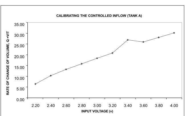
The controlled inflow for every tank also has to be calibrated. It is needed in order to obtain the relationship between the voltage to the pump and the flow rate into the tank. Figure 9 shows the relationship between the voltage to the pump and the flow rate into tank A. From linearization, we obtain the value of kp = 13.29 cm3/
sec/V. Similar step is repeated for tank B and from Figure 10 we get the value of kp
for tank B at 13.43 cm3/sec/V.
0.00 0.50 1.00 1.50 2.00 2.50 3.00 3.50 4.00 4.50 5.00
6 7 8 9 10 11 12 13 14 15 16 17 18 19 20 21 22 23 24 25
CALIBRATING LEVEL SENSOR (TANK A)
LEVEL (cm)
V
O
L
T
A
G
E
(
v
o
lt
s
)
CALIBRATING LEVEL SENSOR (TANK B)
LEVEL (cm)
V
O
L
T
A
G
E
(
v
o
lt
s
2.1.2 Step Response Analysis
In this analysis, step input is given to the system. From the output response obtained, the transfer function of the system is calculated. Figure 11 below illustrates the response of the system with step input.
Five readings are taken for five different graph of step response of first order system. Table 1 shows the readings.
Figure 10 The relationship between the voltage to the pump and the flow rate into the tank B
0.00 5.00 10.00 15.00 20.00 25.00 30.00 35.00
2.20 2.40 2.60 2.80 3.00 3.20 3.40 3.60 3.80 4.00
Figure 9 The relationship between the voltage to the pump and the flow rate into the tank A
INPUT VOLTAGE (v)
R
A
T
E
O
F
C
H
A
N
G
E
O
F
V
O
L
U
M
E
,
Q
=
V
/T
CALIBRATING THE CONTROLLED INFLOW (TANK A)
0.00 5.00 10.00 15.00 20.00 25.00 30.00 35.00 40.00
2.60 2.80 3.00 3.20 3.40 3.60 3.80 4.00 4.20 4.40
INPUT VOLTAGE (volts)
R
A
T
E
O
F
C
H
A
N
G
E
O
F
V
O
L
U
M
E
,
Q
=
V
/T
Figure 11 Step response test of first order system
Table 1 The transfer function obtained from 5 readings taken for Tank A
READING TRANSFER FUNCTION
1
( )
s . e G s s . − = + 10 0 0217 0 0175
2
( )
s . e G s s . − = + 16 0 0332 0 025
3
( )
s . e G s s . − = + 12 0 0221 0 0192
4
( )
s . e G s s . − = + 14 0 0162 0 0167
5
( )
s . e G s s . − = + 14 0 0295 0 0238
Hence, the average transfer function of Tank A is
( )
. s . e G s s . − = + 13 2 0 0245
0 0204 . Table 2 shows five readings taken for Tank B.
A m p li tu d e ( V o lt ) Time (Second) 30.0 27.0 24.0 21.0 18.0 15.0 12.0 9.0 6.0 3.0 0.0
0 50 100 150 200 250 300 350 400 462
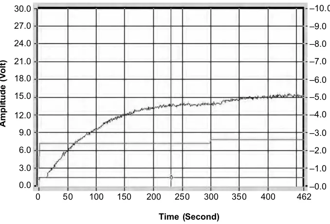
Figure 12 Step response test of second order system
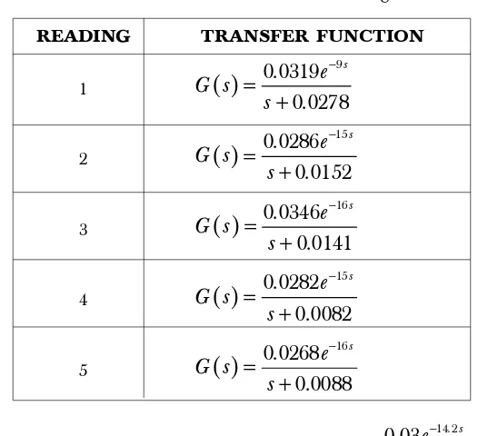
Thus, the average transfer function of Tank B is
( )
. s . e G s s . − = + 14 2 0 03 0 0422.
The experiment is proceeded to second order tank. Step input is applied to Tank A and the output response is observed at Tank B. Figure 12 revealed step response test for 2nd order system.
Table 2 The transfer function obtained from 5 readings taken for Tank B
READING TRANSFER FUNCTION
1
( )
s . e G s s . − = + 9 0 0319 0 0278
2
( )
s . e G s s . − = + 15 0 0286 0 0152
3
( )
s . e G s s . − = + 16 0 0346 0 0141
4
( )
s . e G s s . − = + 15 0 0282 0 0082
5
( )
s . e G s s . − = + 16 0 0268 0 0088 A m p li tu d e ( V o lt ) Time (Second) 30.0 27.0 24.0 21.0 18.0 15.0 12.0 9.0 6.0 3.0 0.0
0 50 100 150 200 250 300 350 400 534
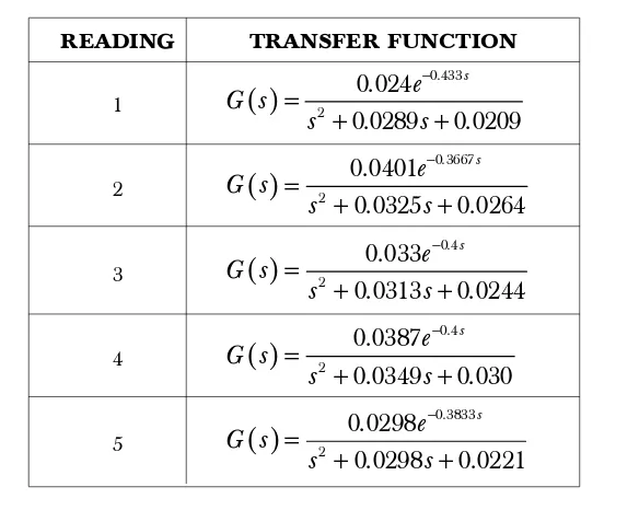
Five readings of second order system test are shown in Table 3.
The average transfer function of 2nd order system is
( )
. s
. e
G s
s . s .
− = + + 0 4 2 0 0331
0 0315 0 0248
2.1.3 Cross Correlation Analysis
In this analysis, pseudorandom binary sequence (PRBS) is injected as input to the system. Pico Scope is used to collect the input and output data of each first order and second order system. Figure 13 illustrates cross correlation graph for first order
Table 3 The transfer function obtained from 5 readings taken for 2nd order system
READING TRANSFER FUNCTION
1
( )
. s
. e
G s
s . s .
− = + + 0 433 2 0 024
0 0289 0 0209
2
( )
. s
. e
G s
s . s .
− = + + 0 3667 2 0 0401
0 0325 0 0264
3
( )
0 4
2
0 033
0 0313 0 0244
. s
. e
G s
s . s .
− =
+ +
4
( )
. s
. e
G s
s . s .
− = + + 0 4 2 0 0387
0 0349 0 030
5
( )
0 3833
2
0 0298
0 0298 0 0221
. s
. e
G s
s . s .
− =
+ +
Figure 13 Cross Correlation of 1st order system
C ro s s c o rr e la ti o n c o e ff ic ie n t Time delay
Cross correlation of first order system
0 50 100 150 200 250 300 350 400 450 500
system. Similar as before, five readings are collected for each system. Table 4 shows five readings taken for first order system.
Thus, the average transfer function for first order system is
( )
. s
. e
G s
s .
− =
+
4 962
1 8667
0 0446 .
Table 4 The transfer function obtained from 5 readings taken for 1st order system
READING TRANSFER FUNCTION
1
( )
. s
. e
G s
s .
− =
+
8 5714
1 5727 0 14
2
( )
. s
. e
G s
s .
− =
+
2 94
1 8182 0 034
3
( )
. s
. e
G s
s .
− =
+
4 55
1 282 0 01
4
( )
. s
. e
G s
s .
− =
+
2 5
1 4243 0 0267
5
( )
. s
. e
G s
s .
− =
+
6 25
2 2364 0 0121
C
ro
s
s
c
o
rr
e
la
ti
o
n
c
o
e
ff
ic
ie
n
t
Time delay
Figure 14 Cross correlation of 2nd order system
Cross correlation of 2nd order system
0 50 100 150 200 250 300 350 400 450
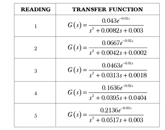
Hence, the average transfer function of second order system obtained through
cross correlation analysis is
( )
. s
. e
G s
s . s .
− = + + 0 018 2 0 1068
0 027 0 0097.
2.1.4 Least Square Method Analysis
Least square method analysis used same collection of data collected from previous analysis. The calculation of that dataset using M-file produces the estimate value of parameters in transfer function of each system. Table 6 shows list of response taken from five readings of first order system.
The average response of first order system obtained from least square method
analysis is y k
( )
. z u k( )
. z − − = + 1 1 0 0107
1 0 9902 .
Table 7 lists five readings of response taken for second order system.
The average response of second order system is
( )
(
. z . z)
( )
y k u k
. z . z
− − − − − + = − − 1 2 1 2
0 0003 0 0122
1 0 564 0 4256 .
Figure 14 revealed cross correlation of second order system whereas Table 5 listed five readings of the system.
Table 5 The transfer function obtained from 5 readings taken for 2nd order system
READING TRANSFER FUNCTION
1
( )
. s
. e
G s
s . s .
− = + + 0 01 2 0 043
0 0082 0 003
2
( )
. s
. e
G s
s . s .
− = + + 0 02 2 0 0667
0 0042 0 0002
3
( )
. s
. e
G s
s . s .
− = + + 0 01 2 0 0463
0 0313 0 0018
4
( )
. s
. e
G s
s . s .
− = + + 0 02 2 0 1636
0 0395 0 0404
5
( )
. s
. e
G s
s . s .
− = + + 0 03 2 0 2136
2.1.4 Controller Design
Two types of controller is designed for each first order and second order system. They are PID family Controller and Fuzzy Logic Controller (FLC).
Table 6 The response obtained from 5 readings taken for 1st order tank
READING RESPONSE
1 y k
( )
. z u k( )
. z − − = + 1 1 0 0017 1 0 9957
2 y k
( )
. z u k( )
. z − − = + 1 1 0 0176 1 0 9813
3 y k
( )
. z u k( )
. z − − = + 1 1 0 0129 1 0 9896
4 y k
( )
. z u k( )
. z − − = + 1 1 0 0102 1 0 9906
5 y k
( )
. z u k( )
. z − − = + 1 1 0 0109 1 0 9937
Table 7 The response obtained from 5 readings taken for 2nd order tank
READING TRANSFER FUNCTION
1 y k
( )
(
. z . z)
u k( )
. z . z
− − − − − + = − − 1 2 1 2
0 0046 0 012 1 0 5454 0 4447
2 y k
( )
(
. z . z)
u k( )
. z . z
− − − − − + = − − 1 2 1 2
0 0068 0 0134 1 0 5367 0 4507
3 y k
( )
(
. z . z)
u k( )
. z . z
− − − − − + = − − 1 2 1 2
0 0045 0 0105 1 0 5725 0 4206
4 y k
( )
(
. z . z)
u k( )
. z . z
− − − − − + = − − 1 2 1 2
0 0070 0 0125 1 0 6087 0 3788
5 y k
( )
(
. z . z)
u k( )
. z . z
− − − − − + = − − 1 2 1 2
2.1.4.1 PID Family Controller
In this stage, four types of PID family controllers are designed. They are Proportional (P) controller, Proportional-Integral (PI) controller, Proportional-Derivative (PD) controller and Proportional-Integral-Derivative (PID) controller. Step input is given to each system and the response for each system with different controllers is recorded and compared with one another.
The transfer function of test system for first order system is
( )
s
. e
G s
s .
− =
+
12
0 034 0 0227. Figure 15 shows the response of the system without any controller.
Figure 15 Response of 1st order system
A
m
p
li
tu
d
e
(
V
o
lt
)
Time (Second)
30.0
27.0
24.0
21.0
18.0
15.0
12.0
9.0
6.0
3.0
0.0
0 50 100 150 200 250 300 350 400 442
0.0 1.0 2.0 3.0 4.0 5.0 6.0 7.0 8.0 9.0 10.0
Figure 16 till 18 shows the response of the system with P, PI and PD controller respectively.
Since the dynamic characteristics of the system is changing, for PID controller,
the test system is
( )
s
. e
G s
s .
− =
+
10
0 051
Figure 17 Response of 1st order system with PI controller
Figure 16 Response of 1st order system with P controller
A
m
p
li
tu
d
e
(
V
o
lt
)
Time (Second)
30.0
27.0
24.0
21.0
18.0
15.0
12.0
9.0
6.0
3.0
0.0
0 20 40 60 80 100 120 140 155
0.0 1.0 2.0 3.0 4.0 5.0 6.0 7.0 8.0 9.0 10.0
A
m
p
li
tu
d
e
(
V
o
lt
)
Time (Second)
30.0
27.0
24.0
21.0
18.0
15.0
12.0
9.0
6.0
3.0
0.0
0 20 40 60 80 100 120 140 168
Figure 18 Response of 1st order system with PD controller
A
m
p
li
tu
d
e
(
V
o
lt
)
Time (Second)
30.0
27.0
24.0
21.0
18.0
15.0
12.0
9.0
6.0
3.0
0.0
0 20 40 60 80 100 120 140 160 209
0.0 1.0 2.0 3.0 4.0 5.0 6.0 7.0 8.0 9.0 10.0
180
Figure 19 Response of 1st order system
A
m
p
li
tu
d
e
(
V
o
lt
)
Time (Second)
30.0
27.0
24.0
21.0
18.0
15.0
12.0
9.0
6.0
3.0
0.0
0 50 100 150 200 250 300 350 400 458
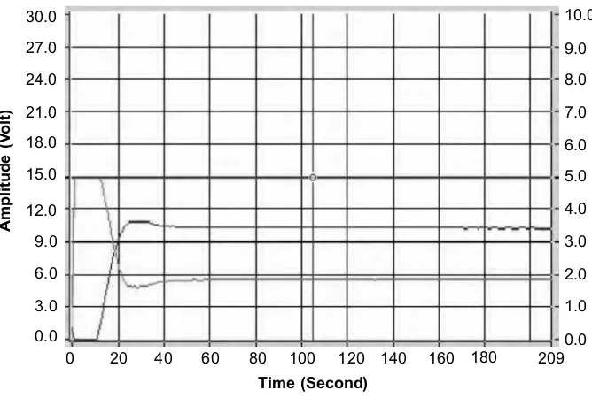
Figure 20 illustrates the response of the system with PID controller.
By observing each graph with different controller, system with PID controller gives the best response compared to others. This is because the system can reach set point with small steady-state error in a short time. In addition, the system settled at steady-state value within small settling time. Other than that, the response shows that the system is stable since there is no overshoot or oscillation. Looking at other controllers, with PI controller, the system reach set point but it is very slow. By having PD controller, response of the system is fast but it cannot reach set point though the value of derivative mode is increased.
For second order system, the transfer function of test system is
( )
. e . sG s
s . s .
− =
+ +
0 3
2
0 0654
0 68 0 7895. The response of the system is illustrated in Figure 21. Figure 22 till 24 each shows the response of the system with P, PI and PD controller respectively.
For PID controller, the test system is
( )
. s
. e
G s
s . s .
− =
+ +
0 2167
2
1 2313
0 870 0 8451. The response can be seen in Figure 25.
Figure 20 Response of 1st order system with PID controller
A
m
p
li
tu
d
e
(
V
o
lt
)
Time (Second)
30.0
27.0
24.0
21.0
18.0
15.0
12.0
9.0
6.0
3.0
0.0
0 20 40 60 80 100 120 140 166
Figure 21 Response of 2nd order system
A
m
p
li
tu
d
e
(
V
o
lt
)
Time (Second)
30.0
27.0
24.0
21.0
18.0
15.0
12.0
9.0
6.0
3.0
0.0
0 25 75 125 175 225 275 325 383
0.0 1.0 2.0 3.0 4.0 5.0 6.0 7.0 8.0 9.0 10.0
50 100 150 200 250 300 350
Figure 22 Response of 2nd order system with P controller
A
m
p
li
tu
d
e
(
V
o
lt
)
Time (Second)
30.0
27.0
24.0
21.0
18.0
15.0
12.0
9.0
6.0
3.0
0.0
0 20 40 60 80 100 120 140 160 177
Figure 24 Response of 2nd order system with PD controller
Figure 23 Response of 2nd order system with PI controller
A
m
p
li
tu
d
e
(
V
o
lt
)
Time (Second)
30.0
27.0
24.0
21.0
18.0
15.0
12.0
9.0
6.0
3.0
0.0
0 20 40 60 80 100 120 140 180
0.0 1.0 2.0 3.0 4.0 5.0 6.0 7.0 8.0 9.0 10.0
A
m
p
li
tu
d
e
(
V
o
lt
)
Time (Second)
30.0
27.0
24.0
21.0
18.0
15.0
12.0
9.0
6.0
3.0
0.0
0 20 40 60 80 100 120 140 180
0.0 1.0 2.0 3.0 4.0 5.0 6.0 7.0 8.0 9.0 10.0
160 202
Figure 25 Response of 2nd order system
A
m
p
li
tu
d
e
(
V
o
lt
)
Time (Second)
30.0
27.0
24.0
21.0
18.0
15.0
12.0
9.0
6.0
3.0
0.0
0 50 100 200 250 350 400 500 565
0.0 1.0 2.0 3.0 4.0 5.0 6.0 7.0 8.0 9.0 10.0
150 300 450
Figure 26 Response of 2nd order system with PID controller
A
m
p
li
tu
d
e
(
V
o
lt
)
Time (Second)
30.0
27.0
24.0
21.0
18.0
15.0
12.0
9.0
6.0
3.0
0.0
0 20 40 60 80 100 120 140 217
0.0 1.0 2.0 3.0 4.0 5.0 6.0 7.0 8.0 9.0 10.0
160 180 200
Figure 27 Response of 1st order system
With P controller, the system cannot reach set point. By having PI controller, the system reach set point but it is very slow. The system gives fast response with PD controller but it cannot reach set point value. Similar as first order system, PID controller give the best performance for the system compared to other controllers. The reason is response of the system reach set point within short time and with small steady-state error. Besides, it settled at steady-state value with small settling time. There also no overshoot and oscillation on the response of the system revealed that the system is stable with this controller.
2.1.4.2 Fuzzy Logic Controller (FLC)
Three types of FLC are used in this paper. They are FLC with 3 × 3 rules, 5 × 5 rules and 7 × 7 rules. The membership chosen is triangular form. Three fuzzy subsets are identified. They are error, E and change of error, ∆E as input to the fuzzy controller whereas change of control signal, ∆U is defined as output from fuzzy logic controller. The performance of FLC with different numbers of rules is compared. Besides, its performance also is compared with PID family controller. The test first order system
for this controller is
( )
s
. e
G s
s .
− =
+
28
2 7435
0 04 . It is illustrated in Figure 27.
A
m
p
li
tu
d
e
(
V
o
lt
)
Time (Second)
30.0
27.0
24.0
21.0
18.0
15.0
12.0
9.0
6.0
3.0
0.0
0 50 100 150 200 250 300 350 475
0.0 1.0 2.0 3.0 4.0 5.0 6.0 7.0 8.0 9.0 10.0
Figure 28 till 30 shows the response of the system with FLC 3 × 3 rules, 5 × 5 rules and 7 × 7 rules respectively.
Figure 28 Response of 1st order system with FLC 3×3 rules
Figure 29 Response of 1st order system with FLC 5×5 rules
A
m
p
li
tu
d
e
(
V
o
lt
)
Time (Second)
30.0
27.0
24.0
21.0
18.0
15.0
12.0
9.0
6.0
3.0
0.0
0 20 40 60 80 100 120 140 232
0.0 1.0 2.0 3.0 4.0 5.0 6.0 7.0 8.0 9.0 10.0
160 180 200 220
A
m
p
li
tu
d
e
(
V
o
lt
)
Time (Second)
30.0
27.0
24.0
21.0
18.0
15.0
12.0
9.0
6.0
3.0
0.0
0 20 40 60 80 100 120 140 240
0.0 1.0 2.0 3.0 4.0 5.0 6.0 7.0 8.0 9.0 10.0
Figure 30 Response of 1st order system with FLC 7×7 rules
By looking at each graph above, FLC with 5 × 5 rules gives the best performance for the system compared to other types of rules. This is because the response is very smooth and there is no oscillation showing that the system is stable. In addition, the system reaches set point within short time with small steady-state error. Its control signal also looks like very smooth. Though the controller with 7 × 7 rules gives zero steady-state error but the response is slower compared to the controller with 5 × 5 rules.
For second order system, the transfer function of the test system is
( )
. e sG s
s . s .
− =
+ +
2
1 3167
0 2 0 8219 . This can be seen in Figure 31.
Figure 32 till 34 shows the response of the system with FLC 3 × 3 rules, 5 × 5 rules and 7 × 7 rules respectively.
From observation, for second order system, in contrast with first order system FLC with 7 × 7 rules gives the best response compared to other different rules. The response is very smooth. The system reaches set point within short time with small steady-state error. Besides, there is no oscillation and its control signal also very smooth.
A
m
p
li
tu
d
e
(
V
o
lt
)
Time (Second)
30.0
27.0
24.0
21.0
18.0
15.0
12.0
9.0
6.0
3.0
0.0
0 20 40 60 80 100 120 140 257
0.0 1.0 2.0 3.0 4.0 5.0 6.0 7.0 8.0 9.0 10.0
Figure 32 Response of 2nd order system with FLC 3×3 rules
Figure 31 Response of second order system
A
m
p
li
tu
d
e
(
V
o
lt
)
Time (Second)
30.0
27.0
24.0
21.0
18.0
15.0
12.0
9.0
6.0
3.0
0.0
0 50 100 150 200 250 300 350 462
0.0 1.0 2.0 3.0 4.0 5.0 6.0 7.0 8.0 9.0 10.0
A
m
p
li
tu
d
e
(
V
o
lt
)
Time (Second)
30.0
27.0
24.0
21.0
18.0
15.0
12.0
9.0
6.0
3.0
0.0
0 20 40 60 80 100 120 140 298
0.0 1.0 2.0 3.0 4.0 5.0 6.0 7.0 8.0 9.0 10.0 400
Figure 33 Response of 2nd order system with FLC 5×5 rules
Figure 34 Response of 2nd order system with FLC 7×7 rules
A
m
p
li
tu
d
e
(
V
o
lt
)
Time (Second)
30.0
27.0
24.0
21.0
18.0
15.0
12.0
9.0
6.0
3.0
0.0
0 20 40 60 80 100 120 140 252
0.0 1.0 2.0 3.0 4.0 5.0 6.0 7.0 8.0 9.0 10.0
A
m
p
li
tu
d
e
(
V
o
lt
)
Time (Second)
30.0
27.0
24.0
21.0
18.0
15.0
12.0
9.0
6.0
3.0
0.0
0 25 50 75 100 125 150 175 347
0.0 1.0 2.0 3.0 4.0 5.0 6.0 7.0 8.0 9.0 10.0
160 180 200 220
3.0 CONCLUSION
Generally, for this system Fuzzy Logic Controller gives better response than PID family controller. It can be seen from the characteristics and the transient response of the system. Response of the system with PID controller is a bit oscillates compared to FLC. FLC is also preferred for this system since it is easier to set up the parameters or the rules to control the system.
REFERENCES
[1] Ljung, L. 1987. System Identification : Theory for The User. 1stedition. United States of America: Prentice Hall.
[2] Benjamin, C. K. 1995. Automatic Control System. 7th Edition. United States of America: John Wiley & Sons, Inc.
[3] Coupled-Tank Liquid Level Computer-Controlled Laboratory Teaching Package: Experimental and Operational (Service) Manual; Augmented Innovation Sdn. Bhd. Centre for Artificial Intelligence and Robotics (CAIRO), Universiti Teknologi Malaysia: Lab Manual.
[4] Norman, S. N. 1995. Control System Engineering. 2nd Edition. Sand Hill Road: Addison-Wesley Publishing Company.
[5] Yeoh Keat Hoe. 2005. System Identification and Parameter Estimation of a Hot Air Blower System Using Nonparametric Methods. Universiti Teknologi Malaysia: Thesis Undergraduate.
[6] Tan Chin Luh. 2001. Application of Direct Digital Control Technique To a Coupled-Tank Apparatus. Universiti Teknologi Malaysia: Thesis Undergraduate.
[7] Eng Yen Lee. 2002. Self-Tuning Control of Coupled-Tank. Universiti Teknologi Malaysia: Thesis Undergraduate.