/umal Tanah dan Lingkungan, Vol. 7 No.2, Oktober 2005: 48-53 ISSN 1410-7333
PREDICTING SPATIAL DISTRIBUTION OF ARGILIC HORIZON
USING AUXILARY INFORMATION IN REGIONAL SCALE
Yiyi
sオQ。・ュ。ョセ@and D. Djaenudin
Soil Research Institute, 98 Juanda st., Bogor, West Java, Indonesia 16123
ABSTRACT
For supporting better soil management, the spatial distribution of soils having argilic hori=on (argilic soils) must be recognized and it can be delineate in soil survey mapping activity, but this activity consumes much time and money. This study aimed to build a decision tree model for predicting the spatial distribution of argillic hori=on based on auxiliary information using 3 predicting environmental variables; namely, geomorphic sUrface or substrate, landsurjace unit, and ecoregion beh. Three-based modeling technique was used to generate classification tree model from 318 pedon of Lampung Province, Indonesia. Argillic horizon is predicted to present in hot belt (elevation of 0-200 m above sea level) on interfluve-seepage slope with probability 84% for acid igneous rock, 83% for basic igneous rock, and 90% for acid sedimentary rock. Argillic horizon is also predicted to present in hot belt on transportational midslope with the probability 65% for transported acid sedimentary rock. Argillic horizon is predicted absent with the probability to occur ranging from 0% to 32% on otlrer combinations of landsurface unit, ecoregion belt, and substrate.
Keywords: Argillic horizon. decision tree, tree-based modeling
INTRODUCTION
The interaction of environmental variables grouped as geological, climatological, biological, and topographical establishes the soil-forming process whose actions on parent material manifest them in soil morphologies which in tum alter the nature of the ongoing process (Chadwick and Graham, 2000). The geological factor constitutes a site factor that sets the initial condition for soil formation, whereas the climatological and biological factors represent energy input that drives soil development. Within any of these factors, local difference in topography modifies the activity of more broadly defined variables. By this understanding, soil surveyor may predict soil properties and their distribution across landscape using such environmental variables.
Many researchers develop model, namely: mathematical equation, decision tree, rules, and neural net, to predict soil properties and their distribution either in local scale or regional scale. They use different predicting environmental variables, approach, technique, target (i.e. a soil property, soil quality, or soil type), and scale (either local scale or regional scale). At regional scale (scale of 1 :250.000 to 1: 100.000), McKenzie and Ryan (1999), for example, used geology, climate, and landscape position as predictors. On the other hand, Chaplot et aI. (2003) used watershed area, landscape position, elevation, and slope, while Sulaeman (2004) used geomorphic surface, landscape position, and elevation as predictors. The characterizing technique of these predictors also varies, for characterizing landscape position, McKenzie and Ryan (1999) and Chap lot et al. (2003) used compound topographic index, whereas Sulaeman (2004) and Park et al. (2001) used Dalrymple model (Dalrymple et al., 1968).
'Alamat korespondensi: Tip. 0251-323012, HP:085220063089, Fax: 0251-321608, e-mail: [email protected]
In addition, some researcher (e.g. Daniels et al., 1971; Carter and Chiolkoz, 1991) prefer to use parametric
technique; but, others (e.g. McKenzie and Ryan, 1999) prefer to use non-parametric one. The parametric approach relies on some assumption; among other, the residual must be normally-distributed with mean of zero, no correlation among predictor, and stable variance. However, soil data do not always satisfy these assumptions. Wilding and Dress (1983) showed that some soil properties follow non-normal distribution. Due to this obstacle, other researchers prefer to use non-parametric approach, such as tree-based modeling technique, generalized additive modeling technique, and Neural Network. However, the selection of which approach will be use depends upon sample number and software availability.
Argillic soil i.e. soils having argillic horizon, mainly of Alfisols and Ultisols (Soil Survey Staff, 1999; Soil Survey Staff, 2003), has dense soil as shown by hard consistency especially of sub soil or diagnostic horimn. These characteristics can limit root penetration and reduce air and water penetration. For example, the infiltration rate of Ultisols under mix garden is about 2.2 cm hour-I and Alfisols is about 1 cm hOUr'l, while the infiltration rate of Andisols is about 3.5 cm hour' 1 (Watung et aI., 2(05). For better soil management, the spatial distribution of argillic soils must be recognized and it can be delineate in soil survey mapping activity, but this activity consumes much time and money (see e.g. Bie and Becket, 1970; Burrough
et al., 1971; Becket, 1981; S ulaeman, 2004). Predicting the occurrence of argillic soil using model may be the other alternative. This model, however, can be built from large soil dataset using data mining technique.
This paper discusses about the modeling of spatial distribution of argiIlic horizon using auxiliary information as predictors. Tree-based modeling is used to develop model since it is non parametric and straightforward to interpret. The resultant model can be used among other to make hypothetical soil map.
Jurnal Tanah dan Lingkungan, Vol. 7 No.2, OktObeT 200S: 48-53
MATERIALS AND METHODS
Dataset
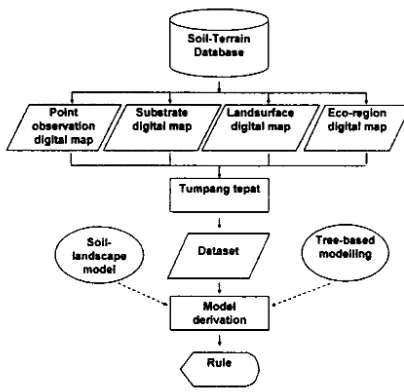
Data for this modeling were extracted from soil and terrain database of Lampung Province (Sulaeman, 2004). Digital map of point observation, subtrate, landsurface, and eco-region were derived and then superimposed to get dataset (Fig. I ). Hence the dataset contains observation code, substrate, landsurface, ecoregion, and the occurrence of argilic subsurface horizon, with the total number 318.
Soli· land.cape
model /
dNセ@
•• t / Iᄋᄋᄋセl⦅mッ、NLMM ..
_I····
セ@ derivation . j
[image:2.599.75.277.215.411.2]c:J
Figure I. Flowchart ofthe Study Table I. Sample Distribution in the Study Area
Explanatory variable Sample number a. Substrate
Sedimentary rock Acid igneous rock Basic igneous rock Acid sedimentary rock
b. Landsurface unit
Interfluve - seepage slope Transportational midslope Colluvial footslope Alluvial toeslope
c. Ecoregion belt
Hot Warm Temperate
318 17
82 133 85
318
83 144
52 39
318
204 87
27
The dataset are predominantly from transportational midslope (144 sample). Based on subtrate, the sample are predominantly developed from basic igeneus rock, while based on eco-region belt, the sample are predominantly taken from hot region (Table I).
Deriving Rule Model
This study derived soil-landscape model which relate environmental variables to soil properties. The soil-landscape model, however, takes advantage of Jenny's soil
formation concept (Jenny, 1954), who consider that the soil properties are controlled by climate, parent material, relief, organism, and time. Other workers ( e.g. McKenzie and Ryan, 1999; Chaplot el ai, 2003) have developed their own soil-landscape model. The principal difference in this model is the expalanatory variable used. This study use substrate, landsurface unit (see Dalrymple el aI., 1968;
Conacher and Dalrymple, 1977; Park el al., 2001),
eco-region belt (see Mohr and van Barren, 1954) as explanatory variables or dependent variables and the occurrence of argilic horizon as independent variable. Sulaeman (2004) formulated the soil-landscape model in mathematical spatial equation as following:
S
=
Gi + Lj + Ek + & where:S = soil (e.g. color, texture, structure, etc),
OJ = i1h substrate, LJ =
t
landsurface,Ek = klh ecoregion belt, and
E = random error factor (e.g. human error, analytical error, etc).
The rule model was derived using tree-based modeling technique based on Classifcation and Regresion Tree (C&RT) algoritm. Other worker have used this technique to get the rule see e.g. The modeling was conducted in PC
computer with the aid of ST A TISTICA (StatSoft Inc, 1999).
RESULTS AND DISCUSSION
Explanatory Variable
The geomorphic surface, landsurface unit, and ecoregion belt represent parent rock/material, relief, and temperature respectively. They can be generated from
auxiliary information i.e. geomorphic surface from geological map, landsurface unit and ecoregion belt from
topographical map. Both geological map and topographical map are available cheaply countrywide. Since they are also mapable, their spatial variability and extent can be recognized.
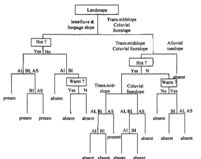
As suggested by classification tree (Fig. 2), landsurface is the first splitting environmental variable of dataset. This indicates that landscape position much
influence on the spatial variability of argillic horizon. The nature of landsurface stability, as shown among other by free from pedoturbation and erosion, may be as source of such variability. Soil formation on interfluve-seepage slope gets free from erosion and produce relatively old soil. In contrast, soil formation on colluvial footslope and alluvial toeslope get much disturbance from erosional and depositional process and produces relatively young soil.
The deviance, however, is lower when ecoregion belt is used as splitting variable (Table 2). For example, the deviance of interfluve decreases 39 % in hot belt, and 27.47 % in warm and temperate belt. This suggests that the combination of landscape position and ecoregion belt is more effective as predictors than landscape position alone.
[image:2.599.60.288.455.618.2]l
I
I
Predicting Spatial Distribution (Y. Su/aeman)
50
presen
1
I
Hot?I
Yes NoAI BI, AS
BI AS
I
LandscapeJ
Interfluve & Seepage slope
AI BI
Warm?
Yes
I
NTrans.midslope Coluvial footslope
Trans.midslope Col uvial footslope
Alluvial toeslope 1..---1....---.
Trans.mid-slope
Hot? Yes
I
NColuvial footslope
I ahsent lWarm . No Yes absent
AI, BI AS AI, BI AS BI AI, AS
presen presen absent absent absent
AI BI AI BI
present absent absent absent
absent absent absent absent
[image:3.602.87.496.58.381.2]Figure 2. Decision Tree for Predicting the Occurrence of Argillic Horizon
Table 2. The Probability of Argillic Horizon to Occur Based on Terrain Information
Terrain attribute Deviance Argillic horizon
Landsurface unit· Ecoregion belt·· Probability (%) Status
1&2 ni·" 112.30 59 present
hot 44.31 84 present
warm or temperate 30.88 19 absent
5,6,7 ni 217.60 17 absent
5,6 hot 143.70 31 absent
5,6 warm or temperate 37.41 6 absent
7 ni 0.00 0 absent
.) 1&2 = Interfluves and seepage slope, 5=transportational midslope, 6=colluvial footslope, 7=alluvial toes lope
•• ) hot = elevation of 0-200 m above sea level (a.s.I), wann = elevation of 200-1 000 m a.s.I, temperate = elevation of 1000-1900 ma.s.1
[image:3.602.81.487.483.621.2]1
I
I
j
'j
1
1
t
1
J
1
-iI
!
i
j
I
J
I
I
J
i
I
I
!
II
I
I
j
I
!
!
,
I
I
!
!
I
I
I
I
I
!Jumal Tanah dan Lingkungan, Vol. 7 No.2, Oktober 2005: 4S-53
The Spatial Occurrence of Argillic Horizon
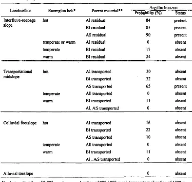
The argillic horizon is predicted present on interfluve-seepage in hot belt (Table 3). Yet, the possibility of argillic horizon to occur differs among parent material. The acid sedimentary rock, including sandstone and claystone, etc. has the highest probability (90%). But, the acid igneous rock including acid tuff, granite, diorite, etc. has the probability of 84%, whereas the basic igneous rock namely basalt, serpentine, etc. has the lowest probability (83%). These result, however, confirm the result of Tafakresnanto and Siswanto (2004) who showed that acidic parent material tends to form argillic-contained soil.
The argillic horizon, however, is predicted absent in colluvial footslope and alluvial toeslope and also in all transported midslope except under hot belt and acid sedimentary parent material. These landscape positions are . unstable surface. Soil formation on these surfaces often get disturbance from either erosion, deposition, mass movement, or the combination of them and produce young non-argillic soils.
Decision Tree
The argillic horizon is also predicted present in transportational midslope and hot belt but only on transported acid sedimentary rock with of 65%, lower than the interfluve has. This also confirms the result of Tafakresnanto and Siswanto (2004). Translocation of clay requires acidic condition or sodic alkaline condition (Buol et ai, 1997). Acid sedimentary rocks, however, contain acid mineral that when they weather produce acid solution (Birkland, 1984).
Figure 2 provides flow chart in predicting the occurrence of argillic horizon as revealed in Table 3. The reading is straightforward. Estimation begins by identifying landscape position in the region. For example, if the landscape position is interfluves-seepage slope according definition in Table 3 and graphic representation in Figure {, then the next question is identified what the ecoregion belt of the site is following the criteria in Table 2. If ecoregion belt is hot, for instance, then the next question is what the parent material is. If parent material is acid igneous rock than the argillic horizon is predicted present in this site.
Table 3. The pprobability of Argillic Horizon to Occur Based on Infonnation of Terrain and Substrate in Lampung Province
Landsurface Ecoregion belt· Parent material·· Probability aアセゥiiゥ」@ (%) horizon Status
Interfluve-seepage hot AI residual 84 present
slope BI residual 83 present
AS residual 90 present
temperate or wann Al residual 0 absent
temperate BI residual 17 absent
wann BI residual 24 absent
Transportational hot AI transported 30 absent
midslope BI transported 32 absent
AS transported 65 present
temperate All transported 0 absent
wann BI transported II absent
AI, AS transported 0 absent
Colluvial foots lope hot AI transported 16 absent
BI transported 22 absent
AS transported 10 absent
temperate All transported 0 absent
wann BI transported II absent
AI • AS transported 0 absent
Alluvial toeslope 0 absent
.) hot = elevation of 0-200 m asl. wann=elevation of 200-1 000 m asl, temperate = elevation of 1000 m asl or higher (see Mohr and van Barren. 1954)
..
) AI = acid igneous rock. BI=basic igneous rocks, AS=acid sedimentary [image:4.604.109.491.360.721.2]Predicting Spatial Distribution (Y. Sulaeman)
Practical Implication
Our result is rules for predicting the spatial occurrence of argillic horizon in Lampung Province on regional scale of 1 :250.000. These rules can be used as a hypothesis of regional scale spatial distribution of argillic horizon in other region having similar environmental condition to Lampung Province. The application of these rules on more detail scale can be accepted as well as landsurface unit can be identified.
The advantage of this rule is that we use predictor that mapable, easily identified on auxiliary information. We can delineate geomorphic surface from geological map. We also can determine ecoregion belt from contour map. Moreover, we can identify landscape position using topographic profile analysis from topographic map. Eventually, we can predict the spatial distribution of argillic horizon in one region. Using this set of rule we can develop hypothetical map that useful in pedological research as well as for other study e.g. ecological study, agriculture, and environmental study).
CONCLUSION
1. Argillic horizon presents in hot belt on interfluve-seepage slope with probability 84% for acid igneous rock, 83% for basic igneous rock, and 90% for acid sedimentary rock.
2. Argillic horizon presents on hot on transportational midslope with the probability 65% for transported acid sedimentary rock.
3. Argillic horizon is absent with the probability to occur ranging from 0% to 32% on other combination of landsurface unit, ecoregion belt, and substrate.
4. Using the decision tree, one may predict the occurrence of argillic horizon in a given region as long as the predictors can be identified.
ACKNOWLEDGEMENT
Authors thank to PAATP project, the Indonesian Department of Agriculture, for partially funding to this research.
REFERENCES
Beckett, P.H.T. 1981. The cost benefits relationship of soil survey. In Soil Resource Inventories and Development Planning. Tech. Monograph No.1. SMSS-SCS. USDA. Washington DC. p. 268-311.
Bie, S.W. and P.H.T. Beckett. 1970. The cost of soil survey. Soils and Fertilizers, 33: 203-217.
Birkeland, P.W. .984. Soils and Geomorphology. Oxford University Press, New York .. 372 pp.
52
Buol, S.W., F.D. Hole, RJ. McCracken, and RJ. Southard. 1997. Soil Genesis and Classification. 4th ed. Iowa State University press, Ames, USA. 527 pp.
Burrough, PA, M.G. Jarvis, and P.H.T. Beckett. 1971. The relationship between cost and utility in soil survey. J. Soil Sci., 22: 359-394, 466-489.
Chadwick, O.A. and R.C. Graham. 2000. Pedogenic processes. In M.E. Sumner (ed.). Handbook of Soil Science. CRC Press,
Boca Raton. p. E41-E75.
Chaplot, V., B. van Vliet-Lanoe, C. Walter, P. Curmi, and M.
Cooper. 2003. Soil spatial distribution in the Annorican Massif, Western France: Effect of soil-forming factors. Soil
Sci., 163:856-868.
Carter, B.J. and E.J. Ciolkosz. 1991. Slope gradient and aspect
effect on soils developed from sandstone in Pennsylvania. Geoderma. 49: 199-213.
Conacher, A.J. and J.B. Dalrymple. 1977. The nine-unit land surface model: and approach to pedogeomorphic rese.c:b.
Geoderma. 18: 1-154.
Dalrymple, J.B., R.J. Blong and AJ. Conacher. 1968. An
hypothetical nine-unit landsurface model. Zeitschr. Fur Geomorph., 12:60-76.
Daniels, R.B, E.E. Gamble and J.G. Cady. 1971. The relation between geomorphology and soil morphology and genesis.
Adv. Agron., 23: 51-88.
Jenny, H. 1941. Factors of Soil Formation: a System of Quantitative Pedology. McGraw-Hili Co, New York.. 281 pp.
Kawtasi, S. 1997. Toposequence of Soil on Diorite Mountain in Benguet, Philippines. [PhD Dissertation] University of the
Philippines, College, Laguna, Philippines. 227 pp.
Lauren, C.P. 1999. Pedological Characterization of Soils Associated with Kennon Limestone. [PhD Dissertation] University of the Philippines, College, Laguna, Philippines. 183 pp.
Mathsoft Inc. 1999. S-Plus Professional Release I. USA.McKenzie, N.J. and PJ. Ryan. 1999. SpItiaI prediction of soil properties using environmental COI1'dIIion.
Geoderma. 89: 67-94.
Mohr, E.C.J. and FA van Baren. 1954. Tropical Soil: a Critical Study of Soil Genesis as Related to Climate, Rock and Vegetation. N.V. Uitgeverij W. Van, The Hague, Netherland. 498 pp.
Park, S.J., McSweeney, and B. Lowery. 2001. IdentifiCllion of the spatial distribution of soils using a process-based terrain characterization. Geoderma, 103 :249-272
Simonson, R.W. 1959. Outline of a generalized theory of soil genesis. Soil Sci. Soc. Am. Proc., 23: 152-156.
Soil Survey Staff. 2003. Keys to Soil Taxonomy. 9'" ed. USDA-NRCS. Washington DC. 332 pp.
Soil Survey Staff. 1999. Soil Taxonomy: A Basic System of Soil Classification for Making and Interpreting Soil Surveys.
Jurnal Tanal! dan Lingkungan, Vol. 7 No.2, Oktober 2005: 48-53
SPSS Inc. 2001. The SPSS C&RT Component: A decision tree component enabling more effective classification and prediction of target variables. CRTWP-OIOI. fip:/ /hafip I.spss.com/pub/web/wp/CRTWP-O I 0 I.pdf. (accessed January 5, 2005, updated April 13,2005). Sulaeman, Y. 2004. A GIS-based Soil Landscape Modeling for
Land Use Planning. [MSc Thesis] University of the Philippines, College, Laguna, Philippines. 183 pp.
Tafakresnanto, C. dan A.B. Siswanto. 2004. Perkembangan Ultisol dan Oxisol dari bahan induk batuan beku dan sediment. In U. Kumia et al. (penyunting). Prosiding Seminar Nasional Inovasi Teknologi Sumberdaya Tanah dan
lklim, Bogor 14-15 Oktober 2003. Puslitbang Tanah dan
Agroklimat. Bogor. p. 139-153.
Watung, L.R., S.H. Tala'ohu, and Ai Dariah. 2005. Landuse change and flood mitigation in Citarum and Kaligarang watershed. In E. Husen, A. Rachman, Irawan, and F.Agus (penyunting). Prosiding Seminar Nasional Multifimgsi Pertanian dan Ketahanan Pangan, Bogor, 12 Oktober - 24 Desember 2004. Puslitbang Tanah dan Agroklimat. Bogor. p.41-54.
Wilding, L.P and L.R. Dress. 1983. Spatial variability and
pedology. In L.P. Wilding, N.E. Smeck and G.F. Hall (cds).
Pedogenesis and Soil Taxonomy: l. Concept and Interaction. Elseiver, Amsterdam. p. 83-116.