LAND COVER CHANGES AND POTENTIAL HYDROLOGICAL
RESPONSES IN PALU CATCHMENT,
CENTRAL SULAWESI
I MADE ANOMBAWA
GRADUATE SCHOOL
BOGOR AGRICULTURAL UNIVERSITY
BOGOR
STATEMENT OF THESIS AND INFORMATION SOURCES
Hereby I declare the thesis entitled Land Cover Changes and Potential Hydrological Responses in Palu Catchment Central Sulawesi Province, is result of my own work under supervision of supervisory committee and it has not been submitted yet in any form in any university to obtain a degree. The researcher has full responsibility for all contents of this thesis. Sources of information derived or quoted from other researchers, whether it is published or not are mentioned in the text and listed in the bibliography at the end of this thesis.
Bogor, August 2012
ABSTRACT
I MADE ANOMBAWA. Land Cover Changes and Potential Hydrological
Responses in Palu Catchment, Central Sulawesi Province. Supervised by PROF.
DR. IR. HIDAYAT PAWITAN, M.SC. as chairman and DR. ANTONIUS B. WIJANARTO as co-supervisor.
In past 20 years the land cover in Palu catchment with total area 3,050 km2 has changed due to the pressure of population activities. This mainly is reducing the amount of forest cover area and increased of urban and agricultural area. It gives impact to the water balance in the catchment, such as the changes of runoff and stream discharges. This study was focused to assess the hydrological response on the stream channel due to the changes of the land use and land cover on the watershed by utilizing remote sensed data, GIS, and hydrological model. Through remote sensing image interpretation, the forest cover has been decreased by 130.6 km2 or equal to 4.3% of total watershed area during period 1990-2001 and 250.9 km2 or equal to 8.2% of total watershed area during period 2001-2009. The conversion of the forest cover is might due to expansion of the agricultural land by 139.2 km2 or 4.6 % during period of 1990 to 2001 and 339.9 km2 or 11.1% during period of 2001 to 2001. From the simulation, it indicated that the total annual discharges volume was increased about 152,390,000 m3 or 4.5% during period 1990 to 2001 and 292,448,000 m3 or 8.2% during period 2001 to 2009. This might due to the changes of land cover and decreased of forest area in Palu Catchment.
ABSTRAK
I MADE ANOMBAWA. Perubahan Penutupan Lahan dan Potensi Respon
Hydrologinya di DAS Palu, Sulawesi Tengah. Di bawah bimbingan dari PROF. DR. IR. HIDAYAT PAWITAN, M.SC. sebagai pembimbing I and DR. ANTONIUS B. WIJANARTO sebagai pembimbing II.
Dalam kurun waktu 20 tahun terakhir, penutupan lahan di DAS Palu dengan luas wilayah 3050 km2 telah mengalami perubahan akibat tingginya tekanan akibat aktifitas penduduk yang tinggal disekitar DAS Palu tersebut. Perubahan ini pada umumnya berkurangnya luah hutan akibat meningkatnya luas lahan pertanian. Hal ini memberikan dampak terhadap neraca air di DAS Palu, seperti meningkatnya aliran permukaan dan debit air. Penelitian ini difokuskan untuk mempelajari perubahan respon hidrologi pada sungai akibat terjadinya perubahan penutupan lahan dengan menggunakan data-data penginderaaan jauh, SIG, dan Model Hidrologi. Berdasarkan hasil interpretasi data citra satelit, luas hutan telah berkurang sebesar 130.6 km2 atau sekitar 4.3% dari luas DAS pada periode 1990-2001, dan 250,9 km2 atau sekitar 8.2% dari keseluruhan luas DAS pada periode 2001-2009. Berkurangnya luas hutan ini diakibatkan oleh bertambahnya luas lahan pertanian sebesar 4.6% dan 11.1% pada periode yang sama. Dari hasil simulasi menunjukan peningkatan jumlah total volume aliran tahunan di DAS Palu sebesar 152.390.000 m3 atau sekitar 4.5% pada tahun 2001 dan 292.448.000 m3 atau sekitar 8.2% pada tahun 2009. Kenaikan total volume aliran tahunan ini kemungkinan besar diakibatkan oleh terjadinya perubahan penutupan lahan dan berkurangnya luas hutan di DAS Palu.
SUMMARY
I MADE ANOMBAWA. Land Cover Changes and Potential Hydrological
Responses in Palu Catchment, Central Sulawesi Province. Supervised by PROF.
DR. IR. HIDAYAT PAWITAN, M.SC. as chairman and DR. ANTONIUS BAMBANG WIJANARTO as co-supervisor.
The increasing of population activities in Palu Catchment is shows by the increasing of the agricultural land and the decreased of forest cover. In a watershed system, forest cover plays important role to maintain the water balances. Forest including the trees and its litters are work to absorb the water when the rain falls down from the sky and store it as ground water. Reduced of forest cover will affected to the forest capacity to absorb the amount of rainfall that will turn the surface runoff increased along with the decreased of forest cover area. If continues, it will lead to deforestation that might to disturb the hydrological system in the watershed. The disruption of the hydrological system is indicated by the increased of peak flow and flood intensity.
Palu City located at the downstream of the Palu Cacthment is mostly flooded in every year. Due to high discharges of Palu River and poor watershed management system makes its occurred frequently and even tended increased by years. It is need serious attention from all stakeholders to makes better watershed management system that can reduce the increased surface runoff. This might be able to be done by conducting reforestation or makes better agricultural system that is can increase the water absorption especially on the upper side of the catchment. The objective of this study is to assess the hydrological response on the stream channel due to the changes of the land use and land covers on its watershed by utilize remote sensed data, GIS, and hydrological model.
impact of land cover changes to hydrological response, three land cover maps of 1990, 2001, and 2009 were used. Besides of those three land cover maps, two different scenarios were employed to find the best scenario’s that is can reduce the surface runoff, the scenarios are; (1) using the Provincial Development Plan (RTRW), and (2) using projected land cover maps on 2020 and 2030.
Trough calibration process 0.81 and 42.9 % of Nash-Sutcliffe coefficient and relative volume error (RVE) was achieved respectively, and 0.758 of R2 of correlation between observed and simulated discharges. During verification process, it gives values 0.9 of Nash-Sutcliffe efficiency and 12.1 % of relative volume errors, with 0.58 of R2 correlation between observed and simulated discharges. This indicated that between observed and simulated discharges using HEC-HMS hydrological model in Palu Catchment have good correlations.
From remote sensing process, can be state that large forest areas have been converted into other land cover classes during period of 1990 to 2009. On land cover period of 1990, 71.3% of total watershed area was covered by forest, 10.7% is used as agricultural land, and 13.6% is shrub land. In 2001 forest cover and shrub land has decreased become 67% and 12.9%, while the agricultural land areas were increased become 15.3%. On 2009 the forest cover and shrub land were reduced significantly become 58.8% and 9.7% respectively, and agricultural land increased to 26.4% of total watershed area. From the hydrological simulations by using rainfall data of 2007 obtained peak discharges about 257.63 m3/s, 268.92 m3/s, and 290.58 m3/s with total discharges 3,422,287 m3, 3,574,677 m3, and 3,867,125 m3 on 1990, 2001, and 2009 respectively.
The total discharges volume of each simulation using different land covers maps was produce 3,422,287,000 m3 on 1990, 3,574,677,000 m3 on 2001, and 3,867,125,000 m3 on 2009. From its simulation found that the discharge volumes were increased 152,390,000 m3 during period 1990 to 2001 and 292,448,000 m3 during period of 2001 to 2009. The contributions of each sub-basin to generate river discharge are difference among sub-basin. Generally, sub-basin 2 gave highest contribution with 31.1% of total discharges was generated, followed by sub-basin 1 with 30.4%, then sub-basin 3 with 13.1%, sub-basin 7 generate about 10% of total discharges, basin 5 with 7.2%, basin 4 with 5.2% and sub-basin 6 with 3.2% respectively.
Copyright © 2012, Bogor Agriculture University Copyright are protected by law,
1. It is prohibited to cite in part or the whole contents of this thesis without referring to and mentioning the sources:
a. Citation only permitted for education purpose, research, scientific writing, report writing, critical writing or reviewing scientific problem.
b. Citation does not inflict the name and honor of Bogor Agricultural University.
LAND COVER CHANGES AND POTENTIAL
HYDROLOGICAL RESPONSES IN PALU CATCHMENT,
CENTRAL SULAWESI PROVINCE
I MADE ANOMBAWA
Thesis is a prerequisite to obtain degree Master of Science in Information Technology for Natural Resources Management Program Study
GRADUATE SCHOOL
BOGOR AGRICULTURAL UNIVERSITY
BOGOR
Research Tittle : Land Cover Changes and Potential Hydrological Responses in Palu Catchment, Central Sulawesi Province.
Student Name : I Made Anombawa
Student ID : G051080071
Study Program : Master of Science in Information Technology for Natural
Resources Management
Approved by, Advisory Board
Prof. Dr. Ir. Hidayat Pawitan, M.Sc Supervisor
Dr. Antonius B. Wijanarto Co-Supervisor
Endorsed by,
Program Coordinator
Dr. Ir. Hartrisari Hardjomidjojo, DEA
Dean of Graduate School
Dr. Ir. Dahrul Syah, M.Sc.Agr
Date of Examination: Date of Graduation:
ACKNOWLEDGEMENT
Thanks to The Almighty God for all of the bless that gave to me, at last this final
project was finished successfully. Sure this research will never complete without
support from various parties: family, colleagues, classmate, MIT secretariat, and
all instance who not able to be mentioned one by one. And through this
opportunity, I would like to express my gratitude to:
1. My beloved families thank you for all of your support, patience, and prayer
during my study.
2. Prof. Dr. Ir. Hidayat Pawitan, M.Sc and Dr. Antonius Bambang Wijanarto, as
supervisor and co-supervisor for all their input, idea, comments, advise, and
all constructive critics during completing my research. I have learned many
things from them.
3. Dr. Surya Darma Tarigan, M.Sc. as my external examiner for his suggestion
to improve my thesis.
4. BMKG, Ministry of Public Work for Water Resources, Bappeda of Central
Sulawesi Province, and BPDAS Palu Poso, for their assistance during field
work and data collection.
5. MIT coordinator, lecturers, and MIT secretariat for their assistance.
6. My classmate of 2008 and all MIT students, for your support and motivation.
7. All others instance that might not able to mention one by one. Thank you for
your support.
I wish that this thesis will give positive contribution to all peoples who read it.
CURRICULUM VITAE
I Made Anombawa was born in Balinggi, Central Sulawesi, Indonesia on
March 14th, 1983, child couple of I Made Subagia and Ni Nengah Derti. He is
second of three brothers. He completed his undergraduate degree in physics at
Tadulako University in 2006. He continued his study in Master of Science in
Information Technology for Nature Resources Management at Bogor Agricultural
University enrolled in 2008, and completed his master degree in 2012. Since
2010, he was working as GIS Coordinator for humanitarian support on disaster
reduction program in one of United Nation Agency that is based in Bandung,
i
2.1 Land Cover Change Detection ... 3
2.1.1 Remote Sensing Application ... 3
2.1.2 Image Classification ... 5
2.1.3 Change Detection ... 6
2.2 Hydrological Characteristic in a Watershed ... 7
2.2.1 Hydrological Cycle ... 7
2.2.2 Watershed Systems ... 8
2.3 Modeling Hydrological Response in a Watershed ... 9
2.3.1 Surface Runoff Estimation ... 10
2.3.2 Unit Hydrograph of Watershed ... 12
III. METHODOLOGY ... 15
3.1 Study Area ... 15
3.1.1 Topography Condition ... 15
3.1.2 Climate Condition ... 16
3.1.3 Land Cover Condition ... 17
3.1.4 Geological Condition ... 17
3.1.5 Demography Condition ... 17
3.2 Data Availability ... 18
3.2.1 Raster and Vector Datasets ... 18
3.2.2 Meteorology and Climate Datasets ... 19
3.2.3 Soil Dataset ... 21
3.2.4 Hydrological Dataset ... 22
3.3 Research Method ... 22
3.3.1 Image Processing ... 24
3.3.1.1 Image Classification ... 24
ii
3.4 Hydrological Modeling ... 26
3.4.1 General Description of HEC-HMS ... 26
3.4.2 Model Parameter and Input ... 28
3.4.2.1 Schematic Watershed Model – Watershed Delineation 28
3.4.2.2 Sub-Basin Lag Time and Peaking Coefficient ... 29
3.4.2.3 Curve Number Determination ... 30
3.4.2.4 Areal Rainfall Estimation ... 31
3.5 Model Calibration and Verification ... 32
3.6 Responses of River System to Land Cover Changes on the Catchment
Area ... 32
IV. RESULTS AND DISCUSSION ... 34
4.1 Land Cover Changes Assessment ... 35
4.1.1 Land Cover Maps from Landsat Data ... 36
4.1.2 Summary of Land Cover Maps ... 39
4.1.3 Change Detection ... 40
4.2 Hydrological Modeling ... 42
4.2.1 Model Input and Parameters ... 42
4.2.1.1 Lag Time and Peaking Coefficient ... 42
4.2.1.2 Curve Number for Surface Runoff Estimation ... 42
4.2.2 Model Calibration and Verification ... 46
4.2.3 Changes in Seasonal Stream Flow ... 48
4.2.4 Response Hydrology to the Land Cover Changes. ... 50
4.2.5 Hydrological Response for some Land Cover Changes
Scenarios. ... 53
4.2.6 Impact of Land Cover Changes Scenarios on Stream Flows .... 55
V. CONCLUSION AND RECOMMENDATIONS ... 59
5.1 Conclusion ... 59
5.2 Recommendation ... 59
REFERENCES ... 61
iii
LIST OF FIGURES
Page Figure 2.1 Hydrological cycles on the earth surface. ... 8
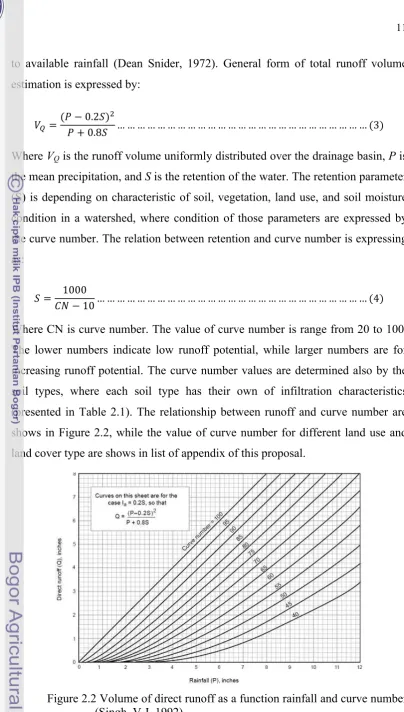
Figure 2.2 Volume of direct runoff as a function rainfall and curve number . 11
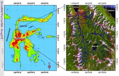
Figure 3.1 Palu Catchment; located in Central Sulawesi. ... 15
Figure 3.2 Digital Elevation Model of Palu Catchment Area ... 16
Figure 3.3 Selected meteorological and hydrological stations ... 20
Figure 3.4 Annual averages rainfall of each rain gauge ... 20
Figure 3.5 Soil map on Palu catchment. ... 21
Figure 3.7 Study workflow. ... 23
Figure 3.8 Image classification processes; four multi temporal images was used to produce land use and land cover classes. ... 25 Figure 3.9. Change detection procedure ... 26
Figure 3.10 Conceptual schematic of the continuous soil moisture model .... 27
Figure 4.1 Satellite imagery of Landsat TM and calculated NDVI. ... 35
Figure 4.2 Land cover map of 1990 and coverage of each land covers class. 37
Figure 4.3 Land cover map of 2001 and Coverage of each land covers class 38
Figure 4.4 Land cover map of 2009 and Coverage of each land covers class.39
Figure 4.5 Increased and decreased of each land cover class ... 39
Figure 4.6 Land use on the Palu catchment ... 41
Figure 4.7 Curve number map of existing land cover on 1990, 2001, and 2009. ... 45
Figure 4.8 Simulation versus observation hydrograph, and correlation
between simulation and observed discharges during calibration process.47
Figure 4.9 Simulation versus observation hydrograph, and correlation between simulation and observed discharges during verification
process. ... 48
Figure 4.10 Twenty years simulated hydrograph in Palu River. ... 49
Figure 4.11. Variations between high wet seasons flow, low dry season flow and peak to low ratio. ... 49
Figure 4.12 Simulated hydrograph from three different lands cover period. . 51
Figure 4.13 Peak stream flow from three different land cover period and Base flow from filtering process for each land cover period. ... 52
v
LIST OF TABLES
Page
Table 2.1 Soil group classification ... 12
Table 3.1 Population on sub-district level across the sub-basin ... 18
Table 3.2 List of used datasets ... 19
Table 3.3 Geographical coordinate of selected hydrology and meteorology observation stations. ... 20
Table 3.4 Metrological station weight calculated using theissen polygon method ... 31
Table 4.1 Summary of land cover maps in Palu Catchment on 1990, 2001, and 2009 ... 39
Table 4.2 Summary of land cover changes in Palu Catchment between period of 1990-2001 and 2001-2009. ... 40
Table 4.3 Change detection statistics report on 1990 – 2001 ... 40
vii
LIST OF APPENDICES
Page
Appendix 1 Runoff curve numbers for urban areas ... 65
Appendix 2 Runoff curve numbers for cultivated agricultural lands ... 66
Appendix 3 Runoff curve numbers for other agricultural lands ... 67
Appendix 4 Runoff curve numbers for arid and semiarid rangelands ... 68
Appendix 5 Observed Discharges ... 69
Appendix 6 Spatial Development Plan of Central Sulawesi Province. ... 72
1
1
I.
INTRODUCTION
1.1 Background
Watershed is the most important factors to maintain the water balance on
the basin area. Watershed with its vegetation including the trees and its litters are
work to absorb the water when the rain falls down from the sky, and store it as
ground water. The increasing of human population is affected to the human need
to land and space either to open new agricultural area or settlement. In developing
countries as well as Indonesia, the land cover changes are mostly issued by the
development of agriculture, residential, and industrial area. Population growth and
their activities to meet the needs are the main driving factors, which lead to the
resources degradation. Land cover changes from forest into agricultural and urban
areas on the watershed system will reduce the capacity of the forest in terms of to
maintain the water supply.
Due to human activities in Palu catchment, large area of forest cover has
been converted into agricultural land in past twenty years. Trough remotely
sensed data; the forest cover has been reduced from 71% in 1990 to 58% of total
watershed area in 2009. It makes the surface runoff increased when the rain
falling down into the catchment. Study of hydrological responses to the land cover
changes enable to assess the sustainability of land use system on the stream river
basin system; because stream flows reflects on the hydrological state of the entire
watershed. Hydrological impact of land cover changes is referencing issues and
must research necessary (Calder, 2002).
Study of hydrological responses to the land cover changes enables us to
assess the sustainability of land use system on the stream river basin system;
because stream flows reflect on the hydrological state of the entire watershed. The
changes of hydrological response due to the land cover changes can be assessed
by integrating appropriately remote sensing data, geographical information system
(GIS), and hydrological models. The results of its integrating method can be
applied to forecast the likely effect of any potential changes in land cover and
2
2
In this study, some analyses were conducted; such as multi temporal
analysis using remote sensing data, hydrological modeling by using hydrological
models tools (HEC-HMS), and GIS for representing the results.
1.2 Problems Statement
Palu catchment area has high density of population. This caused many
effects to the nature resources such as deforestation, changes of forest
management system, overgrazing of the rangeland, and expansion of residential
area and agriculture area. Besides that, the traditional people also do shifting
agriculture system. This shifting agriculture system has significant effect to the
deforestation. Based on last field visit, in last few years some nature hazards such
as flood and landslide happen in this area. Even the last flood hazard is causing
causalities. Besides that, the Palu River also carries out big number of sediment to
the sea, causing pollutant on the sea.
1.3 Objective
This study is aimed to assess the hydrological response on the stream
channel due to the changes of the land use and land cover on its watershed by
3
3
II.
LITERATURE REVIEW
2.1 Land Cover Change Detection
2.1.1 Remote Sensing Application
Remote sensing (RS) usually refers to the technology of acquiring
information about the earth’s surface (land and ocean) and atmosphere, using
sensors onboard airborne (aircraft, balloons) or space-borne (satellites, space
shuttles) platforms (Ranganath et al, 2007). The electromagnetic radiation is
normally used as an information carrier in RS. Remote sensing employs passive
and/or active sensors. Passive sensors are those which sense of natural radiations,
either reflected or emitted from the earth. On the other hand, the sensors are
produce their own electromagnetic radiations are called active sensors. Remote
sensing can also be broadly classified as optical and microwave. In optical remote
sensing, sensors detect solar radiation in the visible, near, middle, and
thermal-infrared wavelength regions, reflected/scattered or emitted from the earth, forming
images resembling photographs taken by a camera/sensor located high up in
space.
Different land cover features, such as water, soil, vegetation, cloud and
snow reflect visible and infrared light in different ways. Interpretation of optical
images requires the knowledge of the spectral reflectance patterns of various
materials (natural or man-made) covering the surface of the earth. It is essential to
understand the effects of atmosphere on the electromagnetic radiation travelling
from the Sun to the Earth and back to the sensor through the atmosphere.
The atmospheric constituents cause wavelength-dependent absorption and
scattering of radiation. These effects degrade the quality of images. Some of the
atmospheric effects can be corrected before the images are subjected to further
analysis and interpretation. A consequence of atmospheric absorption is that
certain wavelength bands in the electromagnetic spectrum are strongly absorbed
and effectively blocked by the atmosphere. The wavelength regions in
electromagnetic spectrum, weather usable for remote sensing, are determined by
4
4
transmission windows. Atmospheric windows used for remote sensing are 0.4-1.3,
1.5-1.8, 2.2-2.6, 3.0-3.6, 4.2-5.0, 7.0-15.0 µm and 10 mm to 10 cm wavelength
regions of the electromagnetic spectrum.
There are also infrared sensors, which measure the thermal infrared
radiation emitted from the earth, from which, the land or sea surface temperatures
and thermal inertia properties can be derived. It is observed that all bodies at
temperatures above zero degrees absolute emit electromagnetic radiation at
different wavelengths, as per Planck’s law, which relates the spectral radiant
emittance E ( , T) with the temperature, T of the object.
! !,! =
the digital number of spectral radiant reflectance of an object in earth surface from
different range of wavelength; where each object have different wavelength
characteristic.
Remote sensing application to land cover changes monitoring is related to
detection process the changes of image in different time period. The land cover
changes from rural to urban condition and the mapping process to land cover
change establishes the baseline to predict to plan water resources, to monitor
adjacent environmentally sensitive areas, and to evaluate development, resource
management, industrial activity, and/or reclamation efforts. The vital component
of mapping is to show the land cover changes in the watershed area and to divide
land use in the various classes of land use. At this stage, remotely sensed imagery
is of great help for obtaining information on temporal trends and spatial
distribution of watershed areas and possible changes over the time dimension for
projecting land cover changes but also to support changes impact assessment.
Furthermore, multi-temporal remotely sensed images are widely considered
5
5 to classify types of land cover, and to obtain a timely regional overview of land
cover information in a practical and economical manner over large areas.
2.1.2 Image Classification
The overall objective of image classification procedures is to automatically
categorize all pixels in an image into land cover classes or themes (Thomas et al.,
2004). Normally, multispectral image are used to perform the classification and,
indeed, the spectral pattern present within the data for each pixel is used as the
numerical basis for categorization. That is, different feature type manifest
different combinations of Digital Numbers (DN) based on their inherent spectral
reflectance and emittance properties. Rather, the terms pattern refers to set of
radiance measurements obtained in the various wavelength bands for each pixel.
Spatial pattern recognition involves the categorization of image pixel on
the basis of their spatial relationship with the pixel surrounding them. Spatial
classifier might consider such aspects as image texture, pixel proximity, feature
size, shape, directionally, repetition, and context. These types of classifiers
attempt to replicate the kind of spatial synthesis done by human analyst during the
visual interpretation processes.
A large number of classification methods are exists which are generally
grouped into two major classification methods; supervised and unsupervised
classification. The classification may either by supervised or unsupervised
classification method. In supervised classification method the pixel categorized
process by specifying, to the computer algorithm, numerical descriptors of the
various land cover types present in an image scene. To do this, representative
sample site of known cover type are used to compile a numerical interpretation
key that describes the spectral attributes of each feature type of interest. Each
pixel in the dataset is then compared numerically to each category in the
interpretation key and labeled with the name of category looks most like. In
unsupervised classification method, the images are first classifying by aggregating
them into the natural spectral groupings present in the image scene. Then the
image analyst determines the land cover identity of these spectral groups by
6
6
To assess the accuracy, the knowledge required to manage territory is
increasingly based on information and maps created from remote sensing images
(Campbell, J.B. 2007; Jensen, J.R. 2005). The accuracy assessment of
classification results is an important feature of land cover and mapping that helps
to determining the quality and reliability of information derived from remote
sensed data. Many factors can be used to assess the accuracy of image
classification results such as classification error matrix and sampling
consideration. Classification error matrices compare, on a category bay category
basis, the relationship between known reference data and the corresponding
results of an automated classification. Sampling consideration is area of
representative, uniform land cover that is different from and considerably more
extensive than training area.
2.1.3 Change Detection
Multi temporal image analysis usually deals with the changes of the
appearance of the object on the earth surface over the time. The differences
between the past and current condition is called the “changes”. These changes
could be the changes of land cover, temperature, land use, rainfall, etc. In terms of
land cover changes, it’s related with to the changes of usage of land in one form to
another form.
Change detection is a process to identifying difference in the state of a
feature by observing it at different moment of time (Singh, 1989). There are large
numbers of change detection algorithm or technique developed and used over the
years to estimate the changes using remote sensing data. The techniques are based
on various mathematical or statistical relationship, principles, and assumption
(Singh, A. 1989). Change detection include image overlay, image digitizing,
image differencing, image regression, image rationing, vegetation index
differencing, principal component analysis, spectral/temporal classification, post
classification comparison, change vector analysis, and background subtraction
(Singh, A 1989; Coppin & Bauer, 1996; Sunar, 1998). Although these methods
have been successful applied in monitoring changes for several applications, there
7
7 detection method employed largely depend on data availability, the geographic
area of study, time and computing constraint, and type of application.
To determinate the land cover changes in past 20 years in the study area,
post classification and matrix analysis have been employed to detect amount of
the changes of each land cover classes. Post classification comparison method
gives us advantages, since this method bypasses the difficulties associated with
the analysis of the multi temporal images or image that came from different
sensors (Alphan, 2003 in Kebede, 2009). This perhaps the most common
approach to assess change detection, and the method comparison uses separate
classification of multi temporal images to produce different maps which is contain
“from-to” information can be generated (Jensen, 2004).
Matrix analysis also called transitional matrix is comparing the area of
each classes from one image to another image. This produces thematic layer
which is contain of information of number of pixel of each classes from two
different images.
2.2 Hydrological Characteristic in a Watershed
2.2.1 Hydrological Cycle
Hydrological cycles are related to the movement of the water from above,
below, and on the earth surfaces. The water on the Earth’s surface; surface water
occurs as streams, lakes, and wetlands, as well as bays and oceans. Surface water
also includes the solid forms of water; snow and ice. The water below the surface
of the Earth primarily is ground water, but it also includes soil water (Winter, T.C.
et al. 1998). The hydrologic cycle commonly is portrayed by a very simplified
diagram that shows only major transfers of water between continents and oceans.
The hydrological cycles consist of precipitation, evaporation, transpiration,
infiltration, percolation, and runoff. Precipitation, which is the source of virtually
all freshwater in the hydrologic cycle, falls nearly everywhere, but the water
distribution, is highly variable. Similarly, evaporation and transpiration return
water to the atmosphere nearly everywhere, but evaporation and transpiration
rates vary considerably according to climatic conditions. As a result, much of the
8
8
water is returned to the atmosphere. The relative magnitudes of the individual
components of the hydrologic cycle, such as evapotranspiration, may differ
significantly even at small scales, as between an agricultural field and a nearby
woodland (Winter, T.C. et al. 1998).
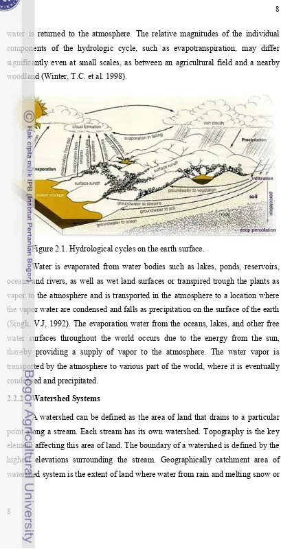
Figure 2.1. Hydrological cycles on the earth surface.
Water is evaporated from water bodies such as lakes, ponds, reservoirs,
oceans and rivers, as well as wet land surfaces or transpired trough the plants as
vapor to the atmosphere and is transported in the atmosphere to a location where
the vapor water are condensed and falls as precipitation on the surface of the earth
(Singh, V.J, 1992). The evaporation water from the oceans, lakes, and other free
water surfaces throughout the world occurs due to the energy from the sun,
thereby providing a supply of vapor to the atmosphere. The water vapor is
transported by the atmosphere to various part of the world, where it is eventually
condensed and precipitated.
2.2.2 Watershed Systems
A watershed can be defined as the area of land that drains to a particular
point along a stream. Each stream has its own watershed. Topography is the key
element affecting this area of land. The boundary of a watershed is defined by the
highest elevations surrounding the stream. Geographically catchment area of
9
9 ice drains downhill into a body of water, such as a river, lake, reservoir, estuary,
wetland, sea or ocean. The drainage basin includes both the streams and rivers that
convey the water as well as the land surfaces from which water drains into those
channels, and is separated from adjacent basins by a drainage divide. The
characteristics of watershed pertain to the land and channel elements of the
watershed. The element of watershed consists of size, shape, slope, elevation,
vegetation, land use, soil type, hydrogeology, lakes, swamps, density of channel,
and artificial drainage (Singh, V.J. 1992).
2.3 Modeling Hydrological Response in a Watershed
Models are considered to simplified representation of real world where
each model has their own conceptual approach, parameters, and related to
mathematical expression. Hydrological models are attempts to represent the
hydrological system from precipitation to stream flow in mathematical form. The
complexity of a hydrological model is varies with the user requirements and the
data availability. Models vary from simple statistical techniques that use graphical
methods for their solution to physically based simulations of the complex
three-dimensional nature of a watershed.
An important issue in modeling the hydrological response of a catchment
is the level of detail at which land cover properties are represented, both where
land cover patterns are stable and where they are changing over time. Nowadays,
various approaches are available to assess the impacts of land cover changes in
different parts of the world. Based on the assessment, most of the hydrological
models belong to the categories of distributed physically based and semi
distributed conceptual hydrological models. In this terminology physically based
stand for the physiographic information of the catchment and climatic factors in a
simplified manner while conceptual stands for the hydrologic state of a catchment,
flows process at any time or instant.
Conceptual rainfall runoff models are normally run with area and average
values of precipitation and evaporation as primary input data and, subject to the
selected approach, produces catchment values of soil-moisture, runoff volumes,
peak flows etc. The conceptual rainfall runoff model is common approach to
10
10
runoff model was applied to assess the hydrological responses to land cover
changes.
2.3.1 Surface Runoff Estimation
Rain that falls into earth surface will experience several processes during
the rainfall process until the water flow to the river. The processes are soil
percolation, and surface runoff. Percolation is process the water infiltrated into the
soil, and surface runoff is the water flow that occurs when the soil is infiltrated
full capacity. The surface runoff happen when the soil is fully infiltrated by the
water. Besides that, surface runoff is very influenced by the soil texture and slope
factors.
Runoff is general term used to indicate the accumulation of precipitation
excess. The volume of runoff is total volume of runoff water occurring over a
period of time. The runoff volume is expressed by integrals of discharge at time
period.
Estimation of runoff volume from a drainage basin involves precipitation,
infiltration, evaporation, transpiration, interception, and depression storage, each
of which is complex and can interact with the other variables to either enhance or
reduce runoff (Singh, V.J. 1992). These variables are variously distributed within
a drainage basin. Actually, to estimate the volume of runoff on drainage basin can
be done by using NRCS Curve Number method.
NRCS Curve Number surface runoff method was introduced by the Soil
Conservation Services United States Department of Agriculture. NRCS curve
number method is an empirical approach parameter used in hydrology for
predicting direct runoff or infiltration from rainfall excess. The runoff curve
number is based on the area's hydrologic soil group, land use, treatment and
hydrologic condition.
The basic concept of this method is the ratio of actual soil retention after
11
11 to available rainfall (Dean Snider, 1972). General form of total runoff volume
estimation is expressed by:
!! =(!− 0.2!)!
!+0.8! … … … …(3)
Where VQ is the runoff volume uniformly distributed over the drainage basin, P is
the mean precipitation, and S is the retention of the water. The retention parameter
(S) is depending on characteristic of soil, vegetation, land use, and soil moisture
condition in a watershed, where condition of those parameters are expressed by
the curve number. The relation between retention and curve number is expressing
as:
!=
1000
!"−10… … … …(4)
Where CN is curve number. The value of curve number is range from 20 to 100.
The lower numbers indicate low runoff potential, while larger numbers are for
increasing runoff potential. The curve number values are determined also by the
soil types, where each soil type has their own of infiltration characteristics
(presented in Table 2.1). The relationship between runoff and curve number are
shows in Figure 2.2, while the value of curve number for different land use and
land cover type are shows in list of appendix of this proposal.
12
12
Table 2.1 Hydrological soil group classifications
Group Soil Characteristics Minimum Infiltration
Rate (in/h)
A Deep sand, deep loess, and aggregate silts 0.3 - 0.45
B Shallow loess and sandy loam 0.15 - 0.30
C Clay loams, shallow sandy loam, soils in organic
content, and soil usually high in clay 0.05 - 0.15
D Soil that swell upon wetting, heavy plastic clay, and
certain saline soils 0 - 0.05
2.3.2 Unit Hydrograph of Watershed
Unit hydrograph of watershed is the direct runoff hydrograph resulting
from one unit of effective rainfall occurring uniformly over the watershed at a
uniform rate during a unit period of time (Singh, V.J. 1992). Actually, the unit
hydrograph is representing the effect of rainfall in particular basin. It is a
hypothetical unit response of the watershed to a unit input of rainfall. The unit
hydrograph firstly developed by Sherman in 1932. Unit hydrograph will use to
determining the surface or direct runoff hydrograph from the effective rainfall
hyetograph (ERH).
The fundamental assumptions implicit in the use of unit hydrographs for
modeling hydrologic systems are:
1. Watersheds respond as linear systems. On the one hand, this implies that the
proportionality principle applies so that effective rainfall intensities (volumes)
of different magnitude produce watershed responses that are scaled
accordingly. On the other hand, it implies that the superposition principle
applies so that responses of several different storms can be superimposed to
obtain the composite response of the catchment.
2. The effective rainfall intensity is uniformly distributed over the entire river
basin.
3. The rainfall excess is of constant intensity throughout the rainfall duration.
4. The duration of the direct runoff hydrograph, that is, it’s time base, is
independent of the effective rainfall intensity and depends only on the
13
13 Hydrologic system is said to be a linear system if the relationship between
storage, inflow, and outflow is such that it leads to a linear differential equation.
The hydrologic response of such systems can be expressed in terms of an impulse
response function through a so-called Convolution Equation. Linear systems
possess the properties of additively and proportionality, which are implicit in the
convolution equation (Ramírez, 2000).
The impulse response function of a linear system represents the response
of the system to an instantaneous impulse of unit volume applied at the origin in
time (t=0). The response of continuous linear systems can be expressed, in the
time domain, in terms of the impulse response function via the convolution
integral as follows,
! ! = !! ! ! !−! !", ℎ ! =0 !"# ! <0 … … … ….(5)
!
!
Where u(t) represents the instantaneous unit hydrograph, and Q(t) and Ie(t)
14
14
15
15
III.
METHODOLOGY
3.1 Study Area
The study area is situated in Palu catchment, Central Sulawesi Province.
Geographically, it is located between 0o52’50” to 1o35’12” S and 119’45’24” to
120’10’50” E.Palu River is the main river that crosses the Palu City and ended in
Palu Bay, study site is show in Figure 3.1. Palu catchment has unique topographic
condition; where in the west and east sides are the mountainous area, while the
north side is hilly and some parts in the southern side is coverage of National
Reserve of Lore Lindu.
Figure 3.1 Palu Catchment; located in Central Sulawesi.
3.1.1 Topography Condition
Palu catchment has unique of topographic characteristic. The elevation of
Palu River Catchment is varying from 0 to 2500 meters above sea level. On the
eastern and western side of Palu River Catchment are hilly areas. As well as the
upstream area of Palu River is a mountainous region that is located in Lore Lindu
16
16
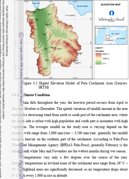
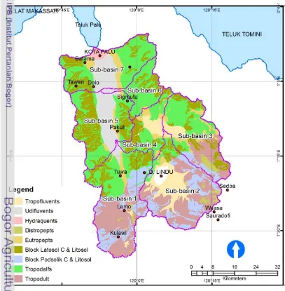
Figure 3.2 Digital Elevation Model of Palu Catchment Area (Sources: SRTM)
3.1.2 Climate Condition
Rain falls throughout the year, the heaviest period occurrs from April to
July and October to December. The spatial variation of rainfall amount in the area
indicated a decreasing trend from north to south part of the catchment area, where
the north side is urban with high population and south part is mountain with high
vegetation. The averages rainfall on the study area is varying depend on the
location with range from 1,000 mm/year – 3,500 mm/year; generally the rainfall
becomes heavier on the southern part of the catchment. According to Palu-Poso
Watershed Management Agency (BPDAS Palu-Poso), generally February is the
driest month while May and November are the wettest months during wet season.
Temperatures vary only a few degrees over the course of the year.
Daytime temperatures in lowland areas of the catchment area range from 26° C –
32° C. Highland areas are significantly decreased, as air temperature drops about
17
17 3.1.3 Land Cover Condition
Based on the topographic map which is issued by the National
Coordinating Agency for Surveys and Mapping (BAKOSURTANAL) now is
Geospatial Information Agency (BIG), in 1991 the land cover composition of Palu
Catchment is dominated by the forest, which is covered more than 70% of total
watershed area, followed by the shrub land, and agricultural land. The forests are
mainly found on the southern part of the catchment, since this area is part of the
Lore-Lindu National Reserves. The main populations were concentrated on the
northern part of the catchment, which is the capital of Central Sulawesi namely
Palu City.
3.1.4 Geological Condition
The geology condition of Palu River Watershed is almost the same for the
overall area. Generally, alluvial soil, innocuous intrusive rocks, metamorphosed
rocks, and sediment compose the geology structures.
The mountainous areas generally consist of acid rock such as gneisses,
schist and granite possessing sensitive to the erosion. The other rock formation,
lacustrine formation can be found on the east side of the study area. On the west
side, alluvium rock that derived from metamorphosed rocks and granite can be
found.
3.1.5 Demography Condition
Demography is important aspect that leads to land cover change in a
catchment area. Most of the changes of the land use are influences by population.
Increasing of the human population means that the needs to the space are
increasing also. Palu Catchment with wit area about 3,050 km2 consists of 13
sub-districts that intersect on the whole catchment area. Where mostly of the
population works as a farmer, which is are utilize a space to farming. Based on the
statistical bureau, the total population that settled in those 13 sub-districts is about
187,535 or 88,763 of households. The demography conditions of study area are
18
18
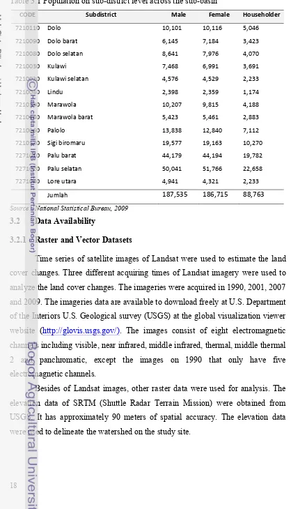
Table 3.1 Population on sub-district level across the sub-basin
CODE Subdistrict Male Female Householder
Source: National Statistical Bureau, 2009
3.2 Data Availability
3.2.1 Raster and Vector Datasets
Time series of satellite images of Landsat were used to estimate the land
cover changes. Three different acquiring times of Landsat imagery were used to
analyze the land cover changes. The imageries were acquired in 1990, 2001, 2007
and 2009. The imageries data are available to download freely at U.S. Department
of the Interiors U.S. Geological survey (USGS) at the global visualization viewer
website (http://glovis.usgs.gov/). The images consist of eight electromagnetic
channels including visible, near infrared, middle infrared, thermal, middle thermal
2 and panchromatic, except the images on 1990 that only have five
electromagnetic channels.
Besides of Landsat images, other raster data were used for analysis. The
elevation data of SRTM (Shuttle Radar Terrain Mission) were obtained from
USGS. It has approximately 90 meters of spatial accuracy. The elevation data
19
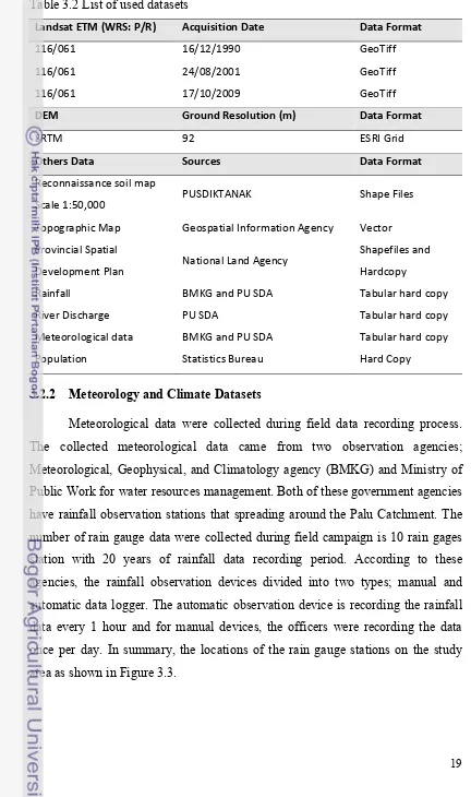
19 Table 3.2 List of used datasets
Landsat ETM (WRS: P/R) Acquisition Date Data Format
3.2.2 Meteorology and Climate Datasets
Meteorological data were collected during field data recording process.
The collected meteorological data came from two observation agencies;
Meteorological, Geophysical, and Climatology agency (BMKG) and Ministry of
Public Work for water resources management. Both of these government agencies
have rainfall observation stations that spreading around the Palu Catchment. The
number of rain gauge data were collected during field campaign is 10 rain gages
station with 20 years of rainfall data recording period. According to these
agencies, the rainfall observation devices divided into two types; manual and
automatic data logger. The automatic observation device is recording the rainfall
data every 1 hour and for manual devices, the officers were recording the data
once per day. In summary, the locations of the rain gauge stations on the study
20
20
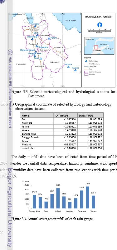
Figure 3.3 Selected meteorological and hydrological stations for Palu Catchment
Table 3.3 Geographical coordinate of selected hydrology and meteorology observation stations.
2009. Besides the rainfall data, temperature, humidity, sunshine, wind speed and
relative humidity data have been collected from two stations with time period of
1990-2009.
21
21 3.2.3 Soil Dataset
The soil types are obtained from Reconnaissance soil map
(PUSLITANAK, 1994). There are 9 kind of soil type found on the study area;
brown alluvial (tropofluvents), grey alluvial (udifluvents), greik alluvial
(hydraquents), cambisol dystrik (distropepts), cambisol eutrik (eutripepts),
litosol-latosol block, podsoic-litosol block, brown litosol-latosol (tropodalfts), and brown
padsolik (trofodulfts). All of these soil types can be categorized into two main
order; inceptisols and ultisols. Inceptisols group can be identified by their texture;
sandy clay, sandy loam clay, clay loam, and loam. This group can be found on
each sub-basin on the study area.
22
22
3.2.4 Hydrological Dataset
Daily series of discharge data of Palu River were collected from
observation station of Ministry of Water Resources (PU-SDA) during the
field-work. There are two of river discharge stations available; one is located near to the
estuary precisely located under Palu II Bridge, and one is located on the upper side of
Palu River. Both of these discharge stations are recording the river discharge once
per day. The collected discharge data were used to validate the model.
Figure 3.6 Daily discharges recorded at Palu River observation station.
Palu Catchment consist of more than 50 river which is can be grouped into five
major group; detail information about its stream network served in figure 3.7 as
below:
Figure 3.7. List of existing river in Palu Catchment (Draft of disaster management plan (RPB) of Palu City, 2009).
0 100 200 300 400 500
2002 2003 2004 2006 2007
Q
(m
3 /s
23
23
3.3 Research Method
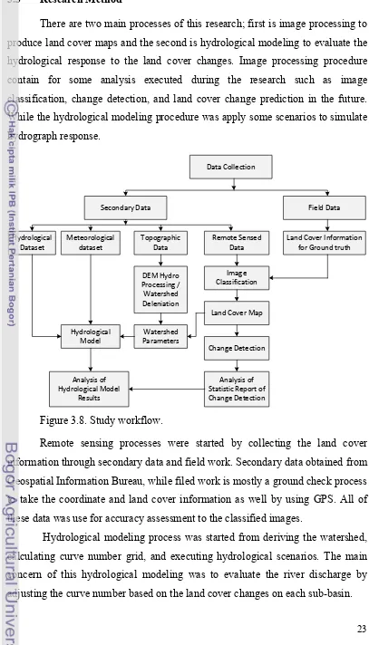
There are two main processes of this research; first is image processing to
produce land cover maps and the second is hydrological modeling to evaluate the
hydrological response to the land cover changes. Image processing procedure
contain for some analysis executed during the research such as image
classification, change detection, and land cover change prediction in the future.
While the hydrological modeling procedure was apply some scenarios to simulate
hydrograph response.
information through secondary data and field work. Secondary data obtained from
Geospatial Information Bureau, while filed work is mostly a ground check process
to take the coordinate and land cover information as well by using GPS. All of
these data was use for accuracy assessment to the classified images.
Hydrological modeling process was started from deriving the watershed,
calculating curve number grid, and executing hydrological scenarios. The main
concern of this hydrological modeling was to evaluate the river discharge by
24
24
3.3.1 Image Processing
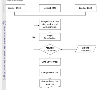
Three different time series images of Landsat were used to identifying the
land cover changes. Those images are Landsat ETM 5 image on 1990, Landsat
ETM+ on 2001, and 2009 of years respectively. The provided images covered
completely all of Palu Catchment area. To ensure that all the images conform to
each other, co-referencing process was done while the 2001 Landsat of year image
was used as baseline image. Co-referencing process is image-to-image
geo-referencing of the images, where one of the images is used as base to geo-correct
other images. Using image geo-referencing method, the maximum allowed of root
mean square error (RMSE) is 0.5 of pixel resolution was achieved, and all of the
images was projected into UTM zone 51S with WGS 1984 datum.
The Landsat images used in this study was acquired from different season,
the atmosphere condition have highly effect to the quality of the images. To
prevent the bad effect of the atmospheric condition, radiometric correction was
done to the all images. The radiometric correction has been done by subtract each
band on the image by its minimum digital number value.
Beside both image co registration and radiometric correction, image
enhancement process was done in this research. Image enhancement is the
improvement process of digital quality on an image. Image enhancement process
was done to get the good image to make easier to identify the object on the
Landsat satellite imageries.
3.3.1.1 Image Classification
Classification is a process to grouping all pixels in an image into certain
classes. Thus, every class can represent an entity with specific properties. Four
time series of Landsat images were used to get the information about land cover
information on the study area. To obtain good accuracy of the land cover classes,
the image was classified through visual interpretation; the land cover
classification flowchart for each Landsat images is shown in Figure 7.
Visual interpretation is utilizing several band combinations to obtain clear
images. Images with Red, Green, and Blue (RGB) combination 542 and 741 are
25
25 RGB images. Visual interpretation procedure is semi-automatic method using on
screen digitizing.
Figure 3.9 Image classification processes; four multi temporal images was used to produce land use and land cover classes.
Visual interpretation was done by observing the pattern of visible object
on the imagery; the object such as river, settlement, and road network are very
helpful to assist us to map the vegetation or land cover. The vegetation mapping is
performed by delineating the outer boundary of pixels that have same pattern, then
it was classified by using an support maps such as land cover maps, topographic,
concessions, and vegetation as a reference maps.
Based on the existing condition of land cover type in study area, the
Landsat images were classed into 6 major classes. The classes are:
1. Forest Land: Area with high density of trees which include primary dry land
forest, secondary dry land forest, swamp forest, mangrove, and plantation
26
26
2. Agriculture: Area used for both annual and perennial crop cultivation, and the
scattered rural settlements are closely associated with the large sized
cultivated field.
3. Shrubs Land: Area covered with shrubs, bushes and small trees, with little
wood mixed with some grasses.
4. Water Body: Area which remains water logged and swampy throughout the
year, the man made dam, the rivers with its main tributaries, and the lake.
5. Build up: Area with high density of settlement that including high density
township residences, and urban area.
6. Barren land: Area dominated by grass and small number of small trees.
3.3.1.2 Change Detection
To identify the differences between two or more land cover maps, post
classification and matrix analysis was performed during image processing stage.
The matrix analysis is comparing the area of each class in each land cover map,
and consists of with two kinds of values; the diagonal matrix contains unchanged
value while the other cell contain with a value that have been changed. Second
step is generating the probability of changes between classes.
Figure 3.10. Change detection procedure (Wijanarto, 2006)
3.4 Hydrological Modeling
3.4.1 General Description of HEC-HMS
HEC-HMS model was designed to simulate the precipitation-runoff
27
27 problems. This includes large river basin water supply and flood hydrology to
small urban or natural watershed runoff. Hydrographs produced by the program
can be used directly or in conjunction with other software for studies of water
availability, urban drainage, flow forecasting, future urbanization impact,
reservoir spillway design, flood damage reduction, floodplain regulation, wetlands
hydrology, and systems operation (Fleming, 2009). HEC-HMS model is a
mathematical model and was designed originally to apply for runoff simulation
and hydrological forecasting.
The main concept of HEC-HMS hydrological model is the use of NRCS
Curve Number process, the model that can be used to assess the availability of
water on a watershed. The NRCS-CN model’s itself describing how the
precipitation entrance to the watershed system through canopy interception, soil
infiltration, percolation, and evapotranspiration. These models also represent the
watershed with a series of storage layer such canopy interception storage, surface
depression storage, upper ground storage, and groundwater storage.
28
28
3.4.2 Model Parameter and Input
3.4.2.1 Schematic Watershed Model – Watershed Delineation
First step in hydrological modeling is delineating watershed boundaries
and discretize to hydrology response unit. The aim of the watershed delineation
process is to determine the boundary of the watershed and also to break it into
smaller management unit (sub-basin) if necessary. The watershed boundary was
derived from Suttle Radar Terrain Mission (SRTM) data with 90 by 90 meters of
spatial resolution. It divided into seven sub-basins as shows in Figure 3.12. In
additional to determining the catchment boundary and its sub-basins area, the
watershed delineation process is also determined the stream network and its
related parameters such as basin slope, river slope, basin distance, river length,
etc. The watershed delineation process was done by using HEC-GeoHMS tool
that is can be integrated as plug-in on ArcMap.
Connector
Reach
Junction
Outlet/Sink
Sub-Basin
29
29
3.4.2.2 Sub-Basin Lag Time and Peaking Coefficient
This research was use the Snyder transform method to transform the
rainfall into unit hydrograph. The Snyder transform method requires the lag time
and peaking coefficient information to determine the peak time. Lag time is
defined as the time difference between the peak of the rain event and the peak
discharge. Based on the Snyder theory, the rainfall transformations into unit
hydrograph are determined by some basin parameter, in which those parameters
can be measured based on the physical form of the watershed (Hartanto, N. 2009).
Figure 3.13 Hydrograph element; lag time illustration.
Basin lag time can be obtained by using some lag time equation. This
study is using Tulsa rural lag time equation, in which the equation was developed
by US Army Corps of Engineers for Tusla district.
!! =!! !
! ! !"# !
!
… … … ….(6)
Where Ct is a coefficient for natural watershed with value 1.420, Tp is lag time, L
is sub-basin length, Lca is length to sub-basin centroid, S is maximum river slope,
and m is a power coefficient with default value of 0.33.
The Snyder peaking coefficient can be calculated by using following
relationship for the peak flow rate that can be used solve for Snyder’s peaking
coefficient.
!! =!!
! !
!
30
30
Where Cp is Snyder peaking coefficient, Qp = 380*Tp-98 and Tp is sub-basin lag
time which is calculated previously. Actually the peaking coefficient can be
adjusted manually to find the best correlation between the observed data and
simulated product.
3.4.2.3 Curve Number Determination
Curve number is a transformation among land cover, soil type, and slope
to represent the amount of surface runoff in a watershed. Curve number method
can use widely and it’s the most efficient method to calculate surface runoff for
single rain event in a watershed. Although the method is designed for a single
storm event, it can be scaled to find average annual runoff values. The stat
requirements for this method are very low, rainfall amount and curve number. The
curve number is based on the area's hydrologic soil group, land use, treatment and
hydrologic condition.
In this research, the curve numbers are obtained by overlaying the land
cover maps, and soil type maps, then the intersection among those three
parameters are gives a numbers based on the curve number look up table which is
developed by Soil Conservation Services (NRCS) – United States Department of
Agricultural (USDA). The calculation of curve numbers were performed using the
equation 4, this described in the literature review section.
The NRCS-CN method does not take into account the effect of slope on
runoff yield. However, there are few models that incorporate a slope factor to CN
method to improve estimation of surface runoff depth and volume (Ebrahimian,
2009). Because of the characteristics of Palu catchment is hilly, slope adjustments
to the curve number was performed by employing the equation as below:
!=
322.79+15.63(!)
!+323.52 … … … ….(8)
Where K is curve number constant, and ! is slope.
The next steps is calculate the sub-basin averages curve number by
employing the weighted averages equation as below:
!"=
!"!!!!
!"#$% !"#$%&'( !"#$… … … …. .… … … …(9)
31
31
3.4.2.4 Areal Rainfall Estimation
The HEC-HMS model requires daily time series precipitation data as the
input. The total of precipitation data from all meteorological stations were located
inside and outside the catchment area is used to estimate the rainfall amount. A
daily areal rainfall of catchment will calculated from daily point measurement of
meteorological stations using Thiessen Polygon Methods.
The Thiessen Polygon is one way of calculating areal precipitation. This
method gives weight to station data in proportion to the space between the
stations. The area of each polygon inside the sub-basin, as a percentage of the
total sub-basin area, is calculated. This factor is then used as the weight of the
station situated within that polygon. The Thiessen weight for each station was
calculated for each sub-basin in Table 3.4. The precipitation for the whole area is
then calculated as follows:
Pj = Rainfall measured at each station
Aj = Area of each polygon inside the basin
Atot = Total sub-basin area
Table 3.4 Metrological station weight calculated using theissen polygon method