KAHROOD MONITORING USING SMALL BASELINE SUBSET SYNTHETIC
APRETURE RADAR (SAR) INTERFEROMETRY
A.Tavakkolia, M.Dehghania
a Dept. of Civil and Environmental Engineering, School of Engineering, Shiraz University, Shiraz, Iran
[email protected]* - [email protected]
KEY WORDS: Kahrood, Landslide, Time series analysis, SAR, Interferometry
ABSTRACT:
The area of Kahrood is a small village located in the north-east of Damavand in the center of the Alborz range, north of Iran. Kahrood is located in Haraz valley exactly below the land slide area. To monitor the temporal evolution of the landslide, the conventional small baseline subset (SBAS), a radar differential Synthetic Aperture Radar interferometry (DInSAR) algorithm is used for time-series analysis. 19 Interferograms characterized by small spatial and temporal baselines are generated using 14 images. In order to remove the topographic effects, a digital elevation model from the Shuttle Radar Topography Mission (SRTM), with a spatial resolution of 90 m, is used. In the time-series analysis the first image was selected as the temporal reference. In the least squares solution, in order to increase the number of observational equation as well as decrease the temporal fluctuations due to atmospheric and unwrapping errors, a smoothing constraint is incorporated into the inversion problem. We divide the deformation time-series into two main parts. The maximum deformation rate estimated from the first part of the time-series is estimated as 3.3 cm within the landslide area. According to the time series results the land surface is moving away from the satellite. The second part of the deformation time-series showed a small landslide rate up to 0.7 cm. According to the time series results the land surface is moving toward the satellite. The deformation is estimated along the Mean line of sight (LOS). Considering the whole time series, the maximum LOS deformation rate is estimated as 14 cm.
1. Introduction
.Interferometry is based on the coherent combination of two or more complex SAR images that recorded by antennas at different locations or times and it has matured to a well-established remote sensing technique over the last 15 years. A landslide is the movement of rock, debris or earth down a slope. They result from the failure of the materials which make up the hill slope and are driven by the force of gravity. Landslides are known also as landslips, slumps or slope failure. The mountainous areas of Iran are mainly subject to landslide. One of these areas, i.e. Kahrood, is located in the Alborz Mountain, northern Iran. The geology map (scale, 1:100,000) of the Kahroud area is shown in Fig. 1. The village of Kahrood is located in the valley exactly below the landslide area. According to Fig 1, the landslide area is surrounded by R3Js rock type including shale, sandstone, siltstone, carbonaceous shale, claystone, quartzite and conglomerate. The south of the area is covered by lava mainly trachyandesitic and trachytic flows. The Barzadeh anticline is passed through the area subject to rock fall while the Panjab anticline is located in the north of the study area. Billions of dollars are lost each year for landslide damage. Thus monitoring of landslides is essential for any warning systems to work efficiently. Interferomeric SAR (InSAR) technique has used to monitor the temporal evolution of the landslide and surface deformation in the Los Angeles, California (Lanari, 2004) and China were especially focused on the Baota landslide (Riedel & Walther, 2008). Billions of dollars are lost each year for landslide damage. Thus monitoring of landslides is essential for any warning systems to work efficiently. SAR Interferometry (InSAR) is a space
path (satellite to ground and back again) between the two image acquisitions. Each interference or fringe shows a 2π change in the wave phase, assigning it a color scale (blue-green-yellow-red) or grey scale. If we assume that the two orbits are coincident (zero baseline), the interferogram should be zero flat if the land remains unchanged. Should any displacement occur over the scenario between the two images acquisitions, an additional distance would appear in the radar signal travel path, resulting in a phase component that can be measured precisely. For the ERS satellites, a change in the line of sight distance of 2.8 cm results in an approximate full 2π phase, and thus a fringe in the interferogram. Thus centimetric ground deformations can be measured with InSAR (Massonnet & Feigl, 1998). However, the orbit distance (baseline) is never zero (because satellites follow different orbits in each pass over the same area), so the interferogram reflects this distance as fringes, which are called topographic fringes. Therefore an interferogram contains topographic and deformation fringes. If we are interested in deformation, topographic fringes must be removed. In our work, a Digital Elevation Model (DEM) was used to remove the topographic fringes. Thus, the interferogram obtained (without topography) only shows deformation fringes, and is called a differential interferogram.
However, InSAR measurements give deformation over distinct time intervals. Time series analysis using a significant number of interferograms enables us to calculate the spatial and temporal characteristics of the deformation (Dehghani, et al., 2009). Therefore, the study of time-varying and long term surface changes would be possible.
The main purpose of this paper is to demonstrate the potential of In-SAR to study the Kahrood landslide. The Kahrood landslide had been monitored with DInSAR algorithm by M. Peyret (Peyret, et al., 2008). In this paper the conventional small baseline subset (SBAS), a radar differential Synthetic Aperture Radar interferometry (DInSAR) algorithm is used for time-series analysis. To reduce the atmospheric effects, orbital errors The International Archives of the Photogrammetry, Remote Sensing and Spatial Information Sciences, Volume XL-1/W5, 2015
and noise associated with unwrapping, a smoothing constraint is incorporated into the time-series analysis.
This paper is organized as follows. Section 2 explains the InSAR time-series analysis algorithm. The time-series results are presented in Section 3. Concluding remarks are presented in section 4.
2. Data and Methods
2.1 Data
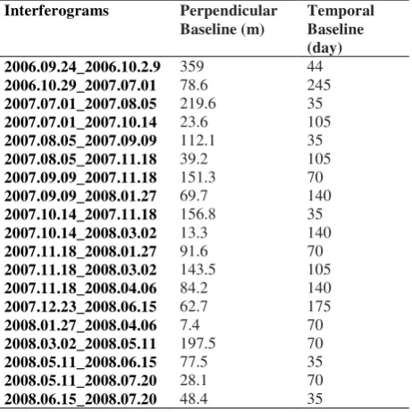
In this study, 14 ENVISAT ASAR raw images provided by ESA spanning between 24 Sep 2006 and 20 Jul 2008 were used. To decrease the spatial and temporal decorrelation problems, the interferograms produced from the Single Look Complex (SLC) ENVISAT ASAR data are characterized by small spatial and temporal baseline. All ENVISAT ASAR data are in IM single look (IMS) mode, with a 9*6 m resolution size in slant and azimuth directions, respectively. 19 Interferograms characterized by small spatial and temporal baselines are generated using 14 images spanning between 2006 and 2008. However, three of them were put aside due to high degree of noise. All the interferograms are calculated using the multilook ratio of 5*1 in azimuth and range direction, respectively, to the squared pixel. Table. 1 illustrates the date of acquisitions of ENVISAT ASAR images and spatial and temporal baselines of the interferograms. In order to remove the topographic effects, a digital elevation model from the Shuttle Radar Topography Mission (SRTM), with a spatial resolution of 90 m, is used.
2.2 Methods
As mention before, Time series analysis enables us to calculate
the spatial and temporal characteristics of the deformation. In this study, InSAR technique was applied to detect and monitor the surface deformation caused by landslide in Kahrood. Small
baseline subset (SBAS) algorithm was used in order to get the deformation rate (Berardio, Fornaro, Lanari, & Sansosti, 2002).
It should be notice that the deformation is estimated along the Mean line of sight (LOS) of the radar satellite by correction factor λ 4�⁄ .
To remove the orbital errors due to the tilts and offsets remaining in the interferograms a plane is fitted to each
interferograms and subtracted from each one (e.g. Funning, Parsons, Wright, & Jachson, 2003).
Table. 1. Constructed interferograms with the spatial and temporal baselines.
Interferograms Perpendicular Baseline (m)
Temporal Baseline (day)
2006.09.24_2006.10.2.9 359 44
2006.10.29_2007.07.01 78.6 245
2007.07.01_2007.08.05 219.6 35
2007.07.01_2007.10.14 23.6 105
2007.08.05_2007.09.09 112.1 35
2007.08.05_2007.11.18 39.2 105
2007.09.09_2007.11.18 151.3 70
2007.09.09_2008.01.27 69.7 140
2007.10.14_2007.11.18 156.8 35
2007.10.14_2008.03.02 13.3 140
2007.11.18_2008.01.27 91.6 70
2007.11.18_2008.03.02 143.5 105
2007.11.18_2008.04.06 84.2 140
2007.12.23_2008.06.15 62.7 175
2008.01.27_2008.04.06 7.4 70
2008.03.02_2008.05.11 197.5 70
2008.05.11_2008.06.15 77.5 35
2008.05.11_2008.07.20 28.1 70
2008.06.15_2008.07.20 48.4 35
The goal of time series analysis is to invert the interferograms to obtain the deformation in each acquisition date by Least-square method. Assume D = [d1 d2 d3 …] is the vector of deformation in each acquisition date that wanted to be estimated and L = [l12 l23 l34 …] is the observation vector that containing the range changes obtained from the interferograms. These vectors are related together by linear equation like eq. (1)
A*D = L, (1)
Where: A= Design matrix L= Observation vector D = Vector of deformation
Fig 1. Geology map of the study area (scale: 1:100,000)
In the inversion solution, the deformation of the first date was set to zero (d1 = 0). In the least squares solution, in order to increase the number of observational equations and increase the degree of freedom, a smoothing constraint is incorporated into the inversion problem. In the other hand to link these 16 interferograms and mitigate several error types, including atmospheric artefacts, noise and unwrapping errors, the smoothing constraint is added into the inversion problem (e.g. Lundgren, et al., 2001; Dehghani et al, 2009). A finite difference approximation for the second-order differential of the time-series are used as a smoothing constraint, eq. (1) is rewritten as:
(Ȣ ���� ��
⁄ ) D = �
� (2)
Where, ȣ is Smoothing factor.
The smoothing factor, ȣ should be determined optimally. The optimal estimation of the smoothing factor has effect in the smooth deformation time-series whereas the non-linear deformation components are preserved. Smoothing factor has effect on time-series results and the time-series results become rough as it is increase. In this case, the observed fluctuations in the results are mostly due to the sources of error in each interferogram. If a large smoothing factor is selected, any non-linear deformation will be damped, and the over weighted smoothing will impose the time-series to be a straight line. If the smoothing is infinite, the best-fit average deformation rate is achieved. Indeed, a trade-off methodology should be applied to select the most appropriate smoothing factor regarding reduction of the errors as well as preservation of the subtle deformation signal. There are several approaches to determine the optimum smoothing factor; one of these is to plot the overall RMS (misfit) that results from least-squares solution against different corresponding smoothing factors. The RMS is the root mean square of the residuals in least-squares solution as follows:
RMS =√∑��= �̂�
� (3)
r̂ = A ∗ D̂ − L (4)
Where �̂ is the estimated phase via least-squares solution.
Fig 2 shows the plot of misfit against smoothing factor and the best smoothing factor. The best smoothing factor is placed in the middle point on the curve where it has a good trade-off between removal of noisy fluctuations and preservation of the nonlinear seasonal deformation. Optimal smoothing factor was then used in all time-series process.
After using the time series analysis to obtain the phase of the deformation in each acquisition date, mean displacement velocity is estimated by dividing the vector of the estimated phases for each pixel to the time interval. Then the estimated values are converted from phase to range.
3. Results
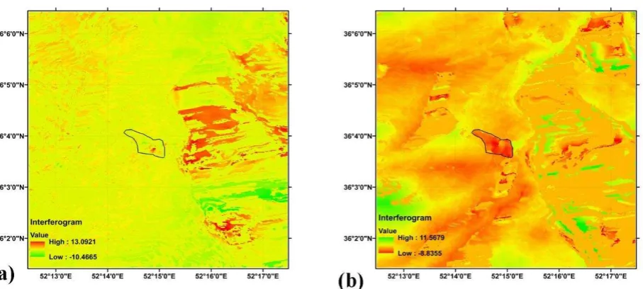
Although some of the interferograms don`t show any changes, in some other interferograms the landslide area can be seen clearly. Fig 3 shows two unwrapped interferograms. The interval covered by the interferograms are: (a) 2007/10/14 to 2008/03/03 and (b) 2008/06/15 to 2008/07/20. They demonstrate very low deformation rate and very high
Fig 3 Two unwrapped interferograms. The interval covered by the interferograms are: (a) 2007/10/14 to 2008/03/03 and (b) 2008/06/15 to 2008/07/20. Black polyline shows the landslide boundary.
Fig 2. Optimum smoothing factor selected at the elbow of the curve. Horizontal and vertical axes represent the smoothing factor and least-squares misfit, respectively.
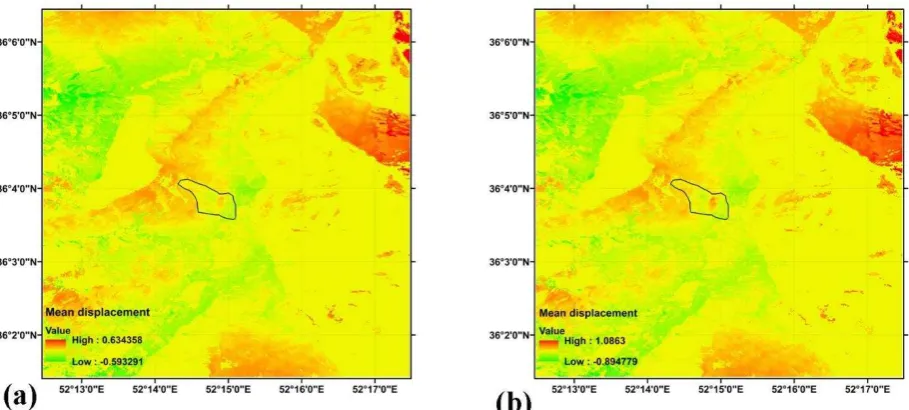
deformation rate in the land slide area, respectively. The landslide area is shown with closest black polyline. As already said, the time series analysis results showed that the area is sliding continuously and does not contain any meaningful seasonal effect. According to the deformation time-series, the deformation rate can be divided into two main parts. The first part spanning between 2006/09/24 and 2007/08/05 shows a decreasing rate. The second part of deformation time-series spanning between 2007/09/09 and 2008/07/20 shows an increasing rate. Fig 4showsmean displacement velocity map. It was computed by using time-series analysis results to the deformation rate and highlight the major deformation features. Deformation area is shown with bright black polyline in Fig 4.
Because of the atmospheric effect in some interferograms, the regions of landslide area in the mean displacement velocity map are not nearly as clear as the other areas.The deformation shown in Fig 4is estimated along the Mean line of sight (LOS). To demonstrate the estimated deformation time-series during the period in each acquisition date, five points were selected in the area. Fig 5shows the distribution of five points in the
land-slide area. Fig 5 shows the time-series deformation of the selected points in two main parts.
According to the parts of mean displacement velocity map, Fig 4 (a) and (b), the mean deformation rates are estimated around 3.3 and 0.7 (cm/yr), respectively. According to the time-series results of first part the land surface is moving away from the satellite and in the second part land surface is moving toward the satellite. The time-series analysis results showed that the area is sliding continuously and does not contain any meaningful seasonal effect.
Fig 4 shows that the landslide area does not have a similar treat. Some parts of the land-slide area, as demonstrated with yellow, have a lower deformation than other parts of the area, as demonstrated with bright orange and green.
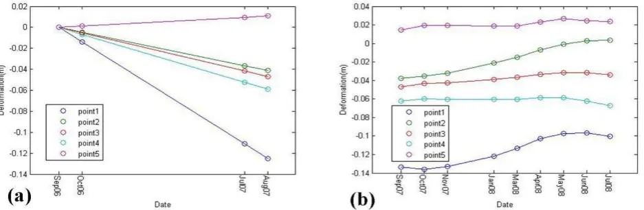
Fig 6 shows the rate of the deformation in landslide area is minus. It means that the land surface is moving away from the satellite continuously. In the first part the deformation rate is very high, Fig 6 (a) and in the other hand in the second part the deformation rate is not nearly as high as first part , Fig 6 (b). So rate of the deformation for each pixel depends to the time and location.
It should be noted that the deformation time series are highly fluctuating in this period probably due to the changes in soil moisture. If we consider whole the time-series, as observed in Fig 6, the maximum LOS deformation rate is about 14 cm yr-1.
4. Conclusions
This paper suggests the conventional small baseline subset (SBAS), a radar differential Synthetic Aperture Radar interferometry (DInSAR) algorithm to monitor the Kahrood landslide. It has been shown to remove the topographic effects due to the non-zeros baselines, a digital elevation model is used. Due to the tilts and offsets that remaining in the interferograms a plane is fitted to each interferograms and subtracted from each one to remove the orbital errors. To decrease the spatial and temporal decorrelation problems, the interferograms produced from the Single Look Complex (SLC) ENVISAT ASAR data are characterized by small spatial and temporal baseline. The Least-square method has been used to calculate the deformation in each acquisition date from interferograms. As already said in Fig 5 Distribution of points in the land-slide area. Five points
are selected in the land-slide area. Black polyline shows the landslide boundary.
Fig 4 (a) The mean displacement velocity map between 2006/09/24 and 2007/08/05; (b) The mean displacement velocity map between 20070909 and 2008/07/20. Black polyline shows the landslide boundary.
order to reduce the atmospheric effects, unwrapping and orbital errors the smoothing constraint have been added into the inversion problem. According to the results, the time-series is divided into the two main parts that the first part shows high decreasing deformation rate and second part shows low deformation rate. The deformation is estimated along the Mean line of sight (LOS).
The mean velocity map of the first part demonstrates the land surface is moving away from the satellite but the second part shows the land surface is moving toward the satellite. The deformation phase was underestimated because of some remain errors such as topography fringes, due to the accuracy of DEM, and atmospheric effects. It should be noted that the deformation time series are highly fluctuating in this period probably due to the changes in soil moisture.
5. Acknowledgements
The authors wish to thank the European Space Agency (ESA) for providing the ENIVSAT ASAR data.
6. References
Berardio, P., Fornaro, G., Lanari, R., & Sansosti, E. (2002). A New Algorithm for Surface Deformation Monitoring. IEEE Trans. on Geoscience and Remote Sensing 40, 2375–2383.
Dehghani, M., Valadan Zoej, M. J., Entezam, I., Mansourian, A., & Saatchi, S. (2009). InSAR monitoring of progressive land subsidence in Neyshabour,. Geophys. J. Int. 178, 47-56.
Dehghani, M., Valadan Zouj, M. J., Saatchi, S., Biggs, J., Parsons, B., & Wright, T. (2009). Radar Interferometry Time Series Analysis of Mashhad Subsidence. J. Indian Soc. Remote Sens., 191-200. Funning, G. J., Parsons, B., Wright, T. J., & Jachson, J. A.
(2003). Surface displacements and source parameters of the 2003 Bam (Iran) earthquake from Envisat advanced synthetic aperture radar imagery. J. geophys. Res.,.
Lanari, R. (2004). Satellite radar interferometry time series analysis of surface. GEOPHYSICAL RESEARCH LETTERS, VOL. 31,. doi:10.1029/2004GL021294 Lundgren, P., Usai, S., Sansosti, E., Lanari, R., Tesauro, M., &
Fornaro, G. &. (2001). Modeling surface deformation observed with SAR. J. geophys. Res., 106, 19 355–19 367.
Massonnet, D., & Feigl, K. L. (1998). RADAR INTERFEROMETRY AND ITS APPLICATION TO. Reviews of Geophysics, 36, 441-500.
Peyret, M., Djamour, Y., Rizza, M., Ritz, J. F., Hurtrez, J. E., Goudarzi, M. A., . . . Uri, F. (2008). Monitoring of the large slow Kahrod landslide in Alborz mountain range (Iran) by. Engineering Geology 100, 131–141. Riedel, B., & Walther, A. (2008). InSAR processing for the
recognition of landslides. Adv. Geosci., 14, 189–194. Fig 6 Deformation time-series of selected points. (a) Deformation time-series of selected points spanning between 2006/09/24 and 2007/08/05. (b) Deformation time-series of selected points spanning between 2007/09/09 and 2008/07/20