CLASSIFICATION OF AIRBORNE LASER SCANNING DATA USING GEOMETRIC
MULTI-SCALE FEATURES AND DIFFERENT NEIGHBOURHOOD TYPES
R. Blomley, B. Jutzi, M. Weinmann
Institute of Photogrammetry and Remote Sensing, Karlsruhe Institute of Technology (KIT) Englerstr. 7, 76131 Karlsruhe, Germany -{rosmarie.blomley, boris.jutzi, martin.weinmann}@kit.edu
Commission III, WG III/2
KEY WORDS:ALS, LiDAR, Point Cloud, Features, Multi-Scale, Classification
ABSTRACT:
In this paper, we address the classification of airborne laser scanning data. We present a novel methodology relying on the use of complementary types of geometric features extracted from multiple local neighbourhoods of different scale and type. To demonstrate the performance of our methodology, we present results of a detailed evaluation on a standard benchmark dataset and we show that the consideration of multi-scale, multi-type neighbourhoods as the basis for feature extraction leads to improved classification results in comparison to single-scale neighbourhoods as well as in comparison to multi-scale neighbourhoods of the same type.
1 INTRODUCTION
Due to the increasing availability of laser scanning systems, more and more data is available in the form of 3D point clouds repre-senting a point-wise sampling of physical object surfaces. Since a user-assisted analysis tends to be quite tedious and costly, an au-tomated analysis of such 3D point clouds is desirable and hence, this automatic analysis has become an important task in pho-togrammetry, remote sensing and computer vision. In this con-text, particular interest has been paid to the detection of specific objects in the acquired data (Pu et al., 2011; Velizhev et al., 2012) and to the classification of each 3D point with respect to pre-defined class labels. For the latter, numerous approaches focus on classifying mobile laser scanning (MLS) data (Munoz et al., 2008; Munoz et al., 2009; Xiong et al., 2011; Hu et al., 2013; Bremer et al., 2013; Weinmann et al., 2015a; Weinmann et al., 2015c) or airborne laser scanning (ALS) data (Chehata et al., 2009; Shapovalov et al., 2010; Shapovalov and Velizhev, 2011; Mallet et al., 2011; Niemeyer et al., 2014; Xu et al., 2014; Guo et al., 2015). While MLS data provide a relatively dense and accu-rate sampling of the considered scene, a significantly lower point density and accuracy may be expected for ALS data. For both types of 3D point cloud data, however, the classification relies on descriptive features which allow an appropriate structural analy-sis and interpretation.
To analyse given 3D point clouds, a variety of approaches has been presented. However, a deeper analysis reveals that most of these approaches may be assigned to one of three major cate-gories. Approaches of the first category focus on a fitting of ge-ometric primitives (e.g. planes, cylinders or spheres) to the data and using the fit parameters as features (Vosselman et al., 2004). Instead of using suchparametric features, the second category of approaches aims to describe the local context by evaluating certain geometric measures (e.g. shape measures represented by a single value which specifies one single property) based on the whole set of 3D points within the local neighbourhood (West et al., 2004; Mallet et al., 2011; Weinmann et al., 2013; Guo et al., 2015). Thesemetrical featuresare to some degree interpretable as they describe fundamental properties of the local neighbour-hood. The third category of approaches focuses on describing the local context by sampling the distribution of a certain met-ric (Osada et al., 2002; Rusu, 2009; Blomley et al., 2014), which
results indistribution features. Meanwhile, especially metrical features and distribution features are widely but separately used for a variety of applications.
While geometric features characterizing the local 3D structure around a considered 3D point may be derived from a respective local neighbourhood, the consideration of multi-scale neighbour-hoods additionally allows to consider the behaviour of the local 3D structure across neighbourhoods of different size. Combin-ing features from multiple scales accounts for the characteris-tic scales of different structures and may hence be beneficial for classification (Brodu and Lague, 2012; Niemeyer et al., 2014; Schmidt et al., 2014; Hu et al., 2013). Yet, in the scope of clas-sifying ALS data, multi-scale neighbourhoods are typically com-posed of local neighbourhoods of the same type (Niemeyer et al., 2014; Schmidt et al., 2014), while the consideration of different neighbourhood types in addition to different neighbourhood sizes may even provide a more promising alternative.
In this paper, we focus on a semantic interpretation of 3D point clouds covering a larger area and we therefore address the point-wise classification of ALS data. We investigate the combined use of metrical features and distribution features as well as the combined use of features from local neighbourhoods of differ-ent scale and type. We perform a thorough analysis of the fea-tures’ and neighbourhoods’ relative and combined performance. In summary, our main contributions consist in
• the extraction of complementary types of geometric features (represented bymetrical featuresanddistribution features),
• the use of different neighbourhood definitions (cylindrical, spherical) for feature extraction, and
• the consideration of metrical features and distribution fea-tures on multiple scales and different neighbourhood types.
2 RELATED WORK
To give an overview of related work, we focus on the different steps which have to be addressed for point cloud classification. First, a local neighbourhood has to be derived for each 3D point to be classified (Section 2.1). Subsequently, those 3D points within the respective local neighbourhood may be used to calculate geo-metric features (Section 2.2), which in turn provide the input for classification (Section 2.3).
2.1 Neighbourhood Selection
The local 3D structure around a considered 3D pointXof a given 3D point cloud is contained in the spatial arrangement of other 3D points within the vicinity ofX. To characterise this local 3D structure, a suitable local neighbourhood has to be specified. In case a single neighbourhood definition is considered as the basis for feature extraction, the features derived provide a single-scale representation of the local 3D structure aroundX. However, features may also be derived from different local neighbourhoods in order to adequately describeX, thus yielding a multi-scale representation. In the following, we summarise the main ideas for both alternatives.
2.1.1 Single-Scale Neighbourhoods: When defining the lo-cal neighbourhood for a given 3D pointX, the first step is to se-lect an appropriate neighbourhood type. In this regard, the most commonly selected neighbourhood types are defined as follows:
• a spherical neighbourhood formed by all 3D points within a sphere aroundX, which is parameterised with a fixed radius (Lee and Schenk, 2002),
• a cylindrical neighbourhood formed by all 3D points within a cylinder whose axis passes throughXand whose radius is fixed (Filin and Pfeifer, 2005), or
• a neighbourhood formed by thek ∈Nnearest neighbours
ofX(Linsen and Prautzsch, 2001).
Note that all these neighbourhood types are parameterised by a single scale parameter (either a radius ork) which is typically selected to be identical for all points of the 3D point cloud. The selected value is derived via heuristic or empiric knowledge about the scene and/or the data. In this context, a smaller scale parame-ter allows to derive features describing fine details of the local 3D structure, whereas a larger scale parameter introduces a certain degree of smoothing and only allows to derive features coarsely describing the local 3D structure. Furthermore, the selection of an appropriate value depends on the sampling rate resulting from data acquisition as well as on the fact that suitable scales may depend on the objects of interest. In order to avoid the use of heuristic or empiric knowledge about the scene and/or the data, it has been proposed to derive a single, but optimal scale for each individual 3D point. Respective approaches mainly rely on the use of a local neighbourhood formed by theknearest neighbours ofX, while the locally optimal scale parameterkoptis derived
via the consideration of the local surface variation (Pauly et al., 2003; Belton and Lichti, 2006), an iterative scheme based on cur-vature, point density and noise of normal estimation (Mitra and Nguyen, 2003; Lalonde et al., 2005), dimensionality-based scale selection (Demantk´e et al., 2011) or eigenentropy-based scale se-lection (Weinmann et al., 2015a; Weinmann, 2016).
2.1.2 Multi-Scale Neighbourhoods: While single-scale neigh-bourhoods allow to derive features which describe the local 3D structure at a specific scale, features derived from multi-scale neighbourhoods additionally allow to describe how the local 3D
geometry behaves across scales (Brodu and Lague, 2012). Yet, respective approaches typically still involve heuristic or empiric knowledge about the scene and/or the data to select suitable val-ues for the different scales (Brodu and Lague, 2012; Niemeyer et al., 2014; Schmidt et al., 2014). Furthermore, features may not only be extracted from one neighbourhood type with a vary-ing scale parameter, but also from different neighbourhood types such as voxels, blocks and pillars (Hu et al., 2013). Again, how-ever, these neighbourhood definitions typically involve heuristic or empiric knowledge about the scene and/or the data.
2.2 Feature Extraction
Once the neighbourhood has been determined for each 3D point, those 3D points within are considered in order to extract respec-tive geometric features. In this context, options are either to ex-tract (i) interpretable features, whereby each feature is typically represented by a single value, or (ii) sampled features, whereby each feature is represented by a collection of values (e.g. in the form of histograms) and single values are hardly interpretable.
2.2.1 Interpretable Features: In order to obtain interpretable geometric features, the spatial arrangement of all points within the local neighbourhood of a respective 3D pointXmay be con-sidered. Based on the 3D coordinates of all these 3D points, it is possible to calculate the 3D covariance matrix which is com-monly referred to as the 3D structure tensor which preserves in-formation about the local 3D structure. More specifically, the eigenvalues of the 3D structure tensor may (i) directly be ex-ploited in order to distinguish between different shape primitives or (ii) be used in order to derive the covariance features of linear-ityLλ, planarityPλ, sphericitySλ, omnivarianceOλ, anisotropy
Aλ, eigenentropyEλand sum of eigenvaluesΣλ (West et al., 2004) and local surface variationCλ(Pauly et al., 2003). The covariance features in particular have been involved in numerous investigations, and they have partially been combined with fur-ther geometric features, e.g. in (Munoz et al., 2008; Weinmann et al., 2013; Guo et al., 2015), or with full-waveform and echo-based features, e.g. in (Chehata et al., 2009; Mallet et al., 2011; Niemeyer et al., 2012; Schmidt et al., 2014).
2.3 Classification
Once features have been derived, the next step is generally to uniquely assign a (semantic) class label to each 3D point of a given 3D point cloud. For this purpose, a supervised classifi-cation is commonly conducted, whereby the strategies of an indi-vidual or a contextual classification may be applied.
2.3.1 Individual Classification: The strategy of an ual classification exploits only the feature vector of each individ-ual 3D pointXto assign a (semantic) class label to this point. This assignment task has been tackled by focusing on very dif-ferent learning principles and therefore involving very difdif-ferent classifiers such as a Maximum Likelihood classifier (Lalonde et al., 2005), an AdaBoost classifier (Lodha et al., 2007), a Random Forest (Chehata et al., 2009), a Support Vector Machine (Mallet et al., 2011) or a Bayesian Discriminant classifier (Khoshelham and Oude Elberink, 2012). While these approaches are relatively efficient and available in numerous software tools, the derived la-belling can be of noisy appearance since no spatial correlation between labels of neighbouring 3D points is taken into account.
2.3.2 Contextual Classification: The strategy of a contextual classification employs the feature vector of the considered 3D pointXas well as the spatial relationship to other neighbouring 3D points in order to assign the (semantic) class label. Among a variety of approaches used for 3D scene analysis are Associative Markov Networks (Munoz et al., 2008; Munoz et al., 2009), non-Associative Markov Networks (Shapovalov et al., 2010; Shapo-valov and Velizhev, 2011) and other inference procedures (Xiong et al., 2011; Shapovalov et al., 2013). Furthermore, it has been proposed to apply Conditional Random Fields on the basis of cylindrical neighbourhoods (Niemeyer et al., 2014; Schmidt et al., 2014) or on the basis of neighbourhoods formed by thek
nearest neighbours (Weinmann et al., 2015b). While such ap-proaches tend to increase the computational burden, they result in a smooth labelling since interactions among neighbouring 3D points are taken into account.
3 METHODOLOGY
In this section, we present our novel methodology for point cloud classification which relies on geometric multi-scale features and different neighbourhood types. The main components of this methodology consist in (i) neighbourhood selection, (ii) feature extraction and (iii) classification, which are explained in the fol-lowing subsections.
3.1 Neighbourhood Selection
As explained in Section 2.1, the first step of 3D scene analysis typically consists in defining appropriate local neighbourhoods as a basis for feature extraction. In this regard, we focus on both single-scale and multi-scale neighbourhoods, and we also con-sider different neighbourhood types as shown in Figure 1.
3.1.1 Single-Scale NeighbourhoodsNc,1m,Nc,2m,Nc,3mand
Nc,5m: In accordance with other investigations focusing on the
classification of airborne laser scanning data, we consider cylin-drical neighbourhoods oriented in vertical direction. For the re-spective scale parameter, i.e. the radius of the cylinder, we use values of1m,2m,3m and5m as proposed in (Niemeyer et al., 2014; Schmidt et al., 2014) for classifying airborne laser scanning data and thus obtain the neighbourhoodsNc,1m, Nc,2m, Nc,3m
andNc,5m.
Ncy
Nk,opt
point of interestX
Figure 1. Concept sketch of neighbourhood definitions used in this work as basis for extracting features for a considered 3D pointX: cylindrical neighbourhood definitionsNcand the
spher-ical neighbourhoodNk,optformed by an optimal numberkoptof
nearest neighbours.
3.1.2 Single-Scale NeighbourhoodNk,opt: Furthermore, we
intend to describe the local 3D structure of each considered 3D pointXbased on a local neighbourhood comprisingXand itsk
nearest neighbours. For this purpose, we involve spatially vary-ing definitions of the local neighbourhood (i.e. varyvary-ing values of the respective scale parameterk), which have proven to be favourable in comparison to identical neighbourhood definitions for all points of the 3D point cloud (Weinmann et al., 2015a; Weinmann et al., 2015b). Particularly eigenentropy-based scale selection (Weinmann et al., 2015a; Weinmann, 2016) has proven to increase the distinctiveness of the geometric features derived from those 3D points within the respective neighbourhood, and we therefore involve eigenentropy-based scale selection in our framework. Accordingly, we use the 3D coordinates of all points within the local neighbourhood in order to derive the 3D struc-ture tensor and its eigenvalues. Subsequently, we normalise these eigenvalues by their sum which results in normalised eigenvalues
λiwithi∈ {1,2,3}and these normalised eigenvalues, in turn, may be used to define the measure of eigenentropy according to
Eλ=−
3
X
i=1
λiln(λi). (1)
By representing this measureEλas a function of the scale pa-rameterk, the main idea of eigenentropy-based scale selection consists in minimizingEλacross varying values ofkwhich cor-responds to minimizing the disorder of 3D points within the local neighbourhood and leads to the optimal scale parameterkoptfor
a considered 3D pointX:
kopt= arg min
k
Eλ(k) (2)
For the involved scale parameterk, we consider all integer num-bers within the interval[10,100]as proposed in (Weinmann et al., 2015a; Weinmann et al., 2015c). The optimum-sized spherical neighbourhoodNk,optis formed by thekoptnearest neighbours
ofX.
3.1.3 Multi-Scale NeighbourhoodNc,all: To also account for
the behaviour of the local 3D geometry across scales, we con-sider a multi-scale neighbourhoodNc,allresulting from the
com-bination of cylindrical neighbourhoods with radii of1m,2m,3m and5m which has also been proposed in (Niemeyer et al., 2014; Schmidt et al., 2014) for classifying airborne laser scanning data.
3.1.4 Multi-Scale, Multi-Type NeighbourhoodNall: We
fi-nally consider a multi-scale neighbourhoodNallresulting from
the combination of the four cylindrical neighbourhoodsNc,1m,
Nc,2m,Nc,3mandNc,5mof varying radii and the spherical
3.2 Feature Extraction
We intend to consider both interpretable features and sampled features, where the described neighbourhood definitions serve as a basis for feature extraction. Shape measures are chosen as in-terpretable features, since they are commonly involved for point cloud classification. For sampled features, we choose shape dis-tributions, since the respective sampling is conducted indepen-dently from a local normal vector, which cannot always be esti-mated reliably for ALS data. Other alternatives such as the spin image descriptor, the 3D shape context descriptor, the SHOT de-scriptor and Point Feature Histograms require such a normal vec-tor (cf. Section 2.2.2).
3.2.1 Shape Measures: To extract descriptive features for a 3D pointXof a considered 3D point cloud, we first extract shape measures in terms of fundamental geometric properties as well as local 3D shape features characterizing the respectively consid-ered local neighbourhood. Note that, in this context, we introduce the term ofshape measuresto describe features that comprise a single value each, whereby the value specifies one (mathemati-cal) property of the whole set of 3D points within the evaluated local neighbourhood.
Among the fundamental geometric properties, we take into ac-count a variety of geometric 3D properties (Weinmann et al., 2015a). These comprise the heightH = Z of the 3D point X, thelocal point densityD derived from the number of 3D points within the local neighbourhood aroundX, and the verti-calityV represented by theZ-component of the eigenvector be-longing to the smallest eigenvalue of the 3D structure tensor. Fur-thermore, we derive themaximum height difference∆Hand the standard deviation of height valuesσHfrom all points within the respectively considered 3D neighbourhood. In case of spherical neighbourhoods whose scale parameter has been determined via eigenentropy-based scale selection, we additionally consider the radiusRof the considered local neighbourhood.
Among the local 3D shape features, we focus on the use of co-variance features(West et al., 2004; Pauly et al., 2003) which are derived from the eigenvalues of the 3D structure tensor, where
λ1≥λ2≥λ3≥0:
Linearity: Lλ=
λ1−λ2
λ1
(3)
Planarity: Pλ=
λ2−λ3
λ1
(4)
Sphericity: Sλ=
λ3
λ1
(5)
Omnivariance: Oλ= 3
v u u t
3
Y
i=1
λi (6)
Anisotropy: Aλ=
λ1−λ3
λ1
(7)
Eigenentropy: Eλ=−
3
X
i=1
λiln(λi) (8)
Sum of eigenvalues: Σλ=
3
X
i=1
λi (9)
Local surface variation: Cλ=
λ3 3
P
i=1
λi
(10)
3.2.2 Shape Distributions:Originally, shape distributions have been introduced as a parameterisation of overall object shape in (Osada et al., 2002). An adaptation of shape distributions as
features for airborne laser scanning point cloud classification is given in (Blomley et al., 2014). In this paper, we follow the im-plementation of the aforementioned reference.
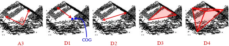
Shape distributions are histograms ofshape values, which are de-rived from random point samples by applying five (distance or angular) metrics (cf. Figure 2). These metrics are:
• A3: the angle between any three random points,
• D1: the distance of one random point from the centroid of all points within the neighbourhood,
• D2: the distance between two random points,
• D3: the square root of the area spanned by a triangle be-tween three random points, and
• D4: the cubic root of the volume spanned by a tetrahedron between four random points.
In order to use shape distributions as features in supervised classi-fication, a fixed number of feature values has to be produced in a repeatable manner. Since the histogram counts of randomly sampledshape valueswithin each local neighbourhood consti-tute the feature values, appropriate histogram binning thresholds and a matching (large enough) number of random pulls are cru-cial prerequisites. Following (Blomley et al., 2014), we choose
10histogram bins, meaning that10feature values will be pro-duced from each metric, and255as the number of pulls from the local neighbourhood. The binning thresholds of the histogram are estimated from the data prior to feature calculation in an adaptive histogram binning procedure. For this purpose,500exemplary local neighbourhoods are first evaluated in a fine-grained linear binning scope. Based on this fine-grained linearly-binned his-togram, a transformation function to a non-linear binning scope with fewer bins is found in such a way that this large number of random samples produces even histogram count values.
3.3 Feature Normalisation
Based on the explanations on feature extraction, it becomes ob-vious that the extracted features address different quantities and therefore have different units as well as a different range of val-ues. Accordingly, it is reasonable to introduce a normalisation allowing to span a feature space where each feature contributes approximately the same, independent of its unit and its range of values. Hence, we conduct a normalisation of both shape mea-sures and shape distributions. For the analytic shape meamea-sures, a linear mapping to the interval between0and1is applied. To avoid the effect of outliers, the range of the data is determined by the1st- and99th-percentiles of the training data. Only if the absolute minimum is zero, the lower range value is set to zero too. For shape distributions, normalisation is achieved by divid-ing each histogram count by the total number of pulls from the local neighbourhood.
3.4 Classification
A3 D1 D2 D3 D4
θ
COG
Figure 2. Visualisation of the five shape distribution metrics A3, D1, D2, D3 and D4.
are all randomly different from each other and hence, taking the majority vote across the hypotheses of all weak learners results in a generalised and robust hypothesis of a single strong learner. When using decision trees as weak learners, the resulting strong learner represents a Random Forest classifier.
4 EXPERIMENTAL RESULTS
In this section, we provide details on the benchmark dataset used for performance evaluation (Section 4.1), describe the conducted experiments (Section 4.2) and present the results accomplished (Section 4.3).
4.1 Dataset
To examine the experimental performance of features from multi-ple scales and neighbourhood types for urban scene classification in airborne laser scanning data, we use a benchmark dataset pre-sented in (Shapovalov et al., 2010). This dataset is kindly pro-vided by the Graphics & Media Lab, Moscow State University, and is publicly available1.
The dataset has been acquired with the airborne laser scanning system ALTM 2050 (Optech Inc.) and consists of two sepa-rate datasets (which are referred to as GML Dataset A and GML Dataset B), each of which is divided into a training and a test-ing part. For both GML Dataset A and GML Dataset B, a ground truth is available in the form of a point-wise labelling with respect to four semantic classes, namelyground,building,treeandlow vegetation. The GML Dataset A additionally contains 3D points which are assigned to the classcar. An overview of the number of labelled 3D points per class and dataset is given in Table 1.
GML Dataset A GML Dataset B Class Training Testing Training Testing Ground 557 k 440 k 1241 k 978 k Building 98 k 20 k 148 k 55 k
Car 2 k 3 k -
-Tree 382 k 532 k 109 k 111 k Low vegetation 35 k 8 k 47 k 17 k
Σ 1075 k 1003 k 1545 k 1161 k Table 1. Number of labelled 3D points in the training set and in the test set for the two parts of the GML Dataset.
4.2 Experiments
For our experiments, we use different neighbourhood definitions as the basis for feature extraction: (i) cylindrical single-scale neighbourhoods defined byNc,1m, Nc,2m, Nc,3m and Nc,5m,
(ii) a spherical single-scale neighbourhood defined by Nk,opt,
(iii) a multi-scale neighbourhoodNc,allresulting from the
com-bination of the cylindrical neighbourhoodsNc,1m,Nc,2m,Nc,3m
and Nc,5m, and (iv) a multi-scale neighbourhood Nall
result-ing from the combination of the neighbourhoodsNc,1m,Nc,2m,
Nc,3m,Nc,5m andNk,opt. The resulting features are
concate-nated to a feature vector and provided as input for a Random For-est, where we use the implementation available with (Liaw and
1http://graphics.cs.msu.ru/en/science/research/3dpoint/classification
GML Dataset A GML Dataset B
N Shape Meas.
Shape Distr.
Both Shape Meas.
Shape Distr.
Both
Nc,1m 25.21 34.09 35.72 31.87 32.46 36.44 Nc,2m 30.61 42.35 44.48 32.39 35.84 37.21 Nc,3m 32.24 44.76 48.64 31.59 33.39 35.10 Nc,5m 41.64 42.05 50.42 27.59 27.43 28.87 Nk,opt 23.34 32.49 28.28 43.66 27.95 43.96
Nc,all 35.45 48.37 49.61 35.52 38.20 39.54
Nall 57.28 53.93 61.17 59.70 58.31 63.76
Table 2. Cκ(in %) for different neighbourhood definitions and different feature sets.
GML Dataset A GML Dataset B
N Shape Meas.
Shape Distr.
Both Shape Meas.
Shape Distr.
Both
Nc,1m 50.22 56.62 57.88 63.65 65.57 68.60
Nc,2m 55.49 64.07 65.68 64.07 68.76 69.05
Nc,3m 57.70 66.14 69.12 62.92 66.05 66.61
Nc,5m 65.10 63.88 70.76 58.09 59.16 59.44
Nk,opt 41.57 51.82 47.11 74.29 58.68 74.28
Nc,all 60.42 68.92 69.93 66.93 69.79 70.43
Nall 74.33 72.20 76.76 84.49 83.74 86.56
Table 3. OA (in %) for different neighbourhood definitions and different feature sets.
Wiener, 2002). The number of treesNT of the Random Forest is determined via a standard grid search which focuses on test-ing different, heuristically selected values. Furthermore, we take into account that a training set with an unbalanced distribution of training examples per class tends to have a detrimental effect on the training process (Chen et al., 2004) and hence introduce a class re-balancing by randomly selecting an identical number of
NEtraining examples per class to obtain a reduced training set. Thereby, NE = 1000is considered to result in representative training data allowing to classify the considered classes.
First, we focus on a classification based on distinct feature groups (i.e. either shape measures or shape distributions) and, subse-quently, we consider them in combination for the classification task. In order to compare the classification results obtained with the different approaches on point-level, we consider a variety of measures for evaluation on the respective test data: (i) Cohen’s kappa (Cκ), (ii) overall accuracy (OA), (iii) mean class recall (MCR) and (iv) mean class precision (MCP). Furthermore, we involve different measures for class-wise evaluation: (i) recall (REC), (ii) precision (PREC) and (iii)F1-score.
4.3 Results
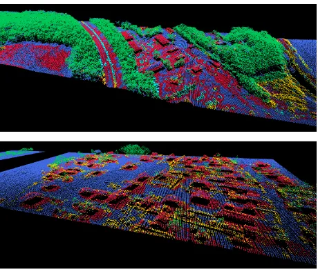
Due to the consideration of seven neighbourhood definitions, three different feature sets and two datasets, a total number of42 ex-periments is conducted. The value of Cohen’s kappaCκand the overall accuracy (OA) for each of these experiments are provided in Table 2 and Table 3. Furthermore, we provide the respec-tive values for mean class recall (MCR) and mean class preci-sion (MCP) in Tables 4 and 5. To obtain an imprespreci-sion on the class-specific properties, the class-wise values for recall (REC) and precision (PREC) are given in Tables 6 and 7. Exemplary classification results are visualised in Figure 3.
im-GML Dataset A GML Dataset B
N Shape Meas.
Shape Distr.
Both Shape Meas.
Shape Distr.
Both
Nc,1m 45.90 52.96 52.73 72.73 69.57 75.14 Nc,2m 49.53 58.77 57.97 72.53 71.73 76.40 Nc,3m 49.34 59.47 60.32 71.96 69.76 74.94 Nc,5m 46.50 56.57 58.17 69.06 64.43 70.66
Nk,opt 36.42 47.44 39.19 74.99 64.33 75.70
Nc,all 51.98 64.84 65.04 76.46 75.15 79.72
Nall 63.48 68.02 70.15 83.47 81.74 85.17
Table 4. MCR (in %) for different neighbourhood definitions and different feature sets.
GML Dataset A GML Dataset B
N Shape Meas.
Shape Distr.
Both Shape Meas.
Shape Distr.
Both
Nc,1m 30.92 36.13 35.58 42.18 41.78 44.84 Nc,2m 32.33 38.20 37.92 43.17 45.35 46.26 Nc,3m 32.49 38.68 38.85 44.41 46.42 46.25 Nc,5m 34.29 38.38 39.28 43.69 42.53 45.02 Nk,opt 35.81 37.50 37.12 50.96 49.65 51.72 Nc,all 33.94 39.83 39.28 45.04 46.68 47.92 Nall 41.64 41.40 43.60 57.11 55.12 58.87
Table 5. MCP (in %) for different neighbourhood definitions and different feature sets.
proved classification results compared to both separate groups. Furthermore, it can be observed that features extracted from multi-scale neighbourhoods of the same type tend to lead to improved classification results. The combination of features derived from multi-scale, multi-type neighbourhoods does, in general, even lead to further improved classification results compared to fea-tures derived from multi-scale neighbourhoods of the same type.
A more detailed view on the derived results reveals that, when considering the evaluation among the single scales, there is no clearbest neighbourhood scaleamong the cylindrical neighbour-hoodsNc,1m, Nc,2m, Nc,3m andNc,5m. For shape measures,
Nc,5m (GML Dataset A) andNc,2m (GML Dataset B) perform
well in class separability (Table 2) and in overall accuracy (Ta-ble 3). For shape distributions,Nc,3m (GML Dataset A) and
Nc,2m (GML Dataset B) show the best results. The class-wise
classification results reveal that different classes favour a differ-ent neighbourhood size (Tables 6 and 7). Furthermore, it may be stated that the spherical neighbourhoodNk,opt, which is
cho-sen via eigenentropy-based scale selection, behaves differently among the two datasets. On GML Dataset A, the resultingCκ shows that all classification results are below those of cylindrical neighbourhoods, while on GML Dataset B both the shape mea-sures and the combined feature groups lead to superior results in comparison to the respective cylindrical neighbourhoods.
When considering features extracted from multiple scales, we may observe that the features extracted from multiple cylindrical neighbourhoodsNc,allare usually similar to or slightly improved
over the best classification result from the individual neighbour-hoods (Tables 2 and 3). However, since there is a large varia-tion among which neighbourhood size performs best in the two datasets, it seems worthwhile to test all scales.
When considering multi-scale, multi-type neighbourhoods, we may state that – even though the spherical neighbourhood se-lected via eigenentropy-based scale selection does not always perform very well on its own – there is usually a notable per-formance increase for the multi-type combinationNallover all
other neighbourhood types or combinations.
5 DISCUSSION
The main focus throughout this work is to determine the be-haviour of different feature types, namely shape measures as
com-Figure 3. Visualisation of the classification results for GML Dataset A (top) and GML Dataset B (bottom) with the classes ground (blue), building(red), car(cyan),tree (green) andlow vegetation(yellow).
mon representatives of interpretable features and shape distribu-tions as an example of sampled features for neighbourhoods and neighbourhood combinations of different type and scale. This comparison has yielded the following insights.
The results accomplished here are comparable to those results of existing research. The most important possibility of compari-son is to (Shapovalov et al., 2010), where the same two datasets have been used as well as a combination of metrical features and distribution features. While our methodology focuses on an im-proved characterisation of 3D points via feature extraction from local neighbourhoods of different scale and type, the methodol-ogy presented in (Shapovalov et al., 2010) focuses on the use of non-Associative Markov Networks and thus a contextual classi-fication. As our approach only performs point-wise individual classification, we expect that not all results of the contextual classi-fication may be matched. Comparing values of REC and PREC, we find thatgroundperforms similar (on GML Dataset A, our in-ferior REC values are compensated for by a higher PREC, while on GML Dataset B only REC is slightly lower),buildings per-form slightly better in REC, but worse in PREC on both datasets, carin GML Dataset A is detected with much higher REC, but lower PREC,treeis generally comparable (slightly lower REC on GML Dataset A and lower PREC but higher REC on GML Dataset B) andlow vegetationagain shows higher REC, but lower PREC values. Other qualitative comparisons may be sought for the individual feature groups. Overall, the performance is com-parable and gives a positive evaluation of our results, considering that no contextual information is exploited.
Shape distributions have already been used in (Blomley et al., 2014) with cylindrical neighbourhoods for urban scene classifi-cation. There, the class-specific studies of classification perfor-mance across different cylinder radii indicated, that radii of1-2m are suitable forbuildingand tree, while slightly larger radii of about3m are more suited forgroundandlow vegetation. A trans-fer of the class-wise REC and PREC values toF1-scores for the
single-scale neighbourhoods Nc,1m, Nc,2m, Nc,3m and Nc,5m
GML Dataset A GML Dataset B
Nk,opt 43.12 40.07 44.36 72.93 55.16 72.66
Nc,all 57.13 46.38 55.63 63.51 67.00 67.17
Nall 64.57 52.38 62.89 83.82 82.93 86.02 Building
Nc,1m 50.79 43.19 50.61 69.51 54.98 69.55 Nc,2m 50.75 42.52 48.63 71.04 61.54 75.55 Nc,3m 53.18 38.26 48.14 73.18 56.51 75.37 Nc,5m 56.38 39.33 53.75 71.81 52.27 68.61 Nk,opt 62.85 48.89 60.11 66.93 52.11 68.61 Nc,all 60.47 45.70 53.78 80.74 74.05 84.34 Nall 63.82 53.58 64.81 80.58 80.01 84.00
Car Nk,opt 40.13 61.85 49.53 90.60 93.26 92.06
Nc,all 63.56 88.38 82.47 89.53 92.71 91.53
Nall 83.17 89.30 88.92 93.65 94.92 94.10 Low vegetation
Nc,1m 17.83 49.68 30.20 72.59 70.93 75.82 Nc,2m 29.58 59.67 44.11 69.52 70.43 74.94
Nc,3m 27.96 66.56 55.07 65.97 67.31 70.06
Nc,5m 27.31 66.90 59.85 64.44 61.26 69.67
Nk,opt 2.63 40.58 10.40 69.49 56.78 69.45
Nc,all 41.18 70.28 61.70 72.05 66.85 75.86
Nall 60.65 70.52 63.11 75.83 69.11 76.57
Table 6. Class-wise REC (in %) for different neighbourhood def-initions and different feature sets.
A comparison of the classification results derived for cylindri-cal single-scylindri-cale neighbourhoods and multi-scylindri-cale neighbourhoods of the same (cylindrical) type reveals that the behaviour of the local 3D structure across different scales provides information which is relevant for the classification task. This becomes visi-ble in improved classification results for multi-scale neighbour-hoods of the same type. Furthermore, we may state that the different neighbourhood types capture complementary informa-tion about the local 3D structure. This clearly becomes visible in the improved classification results obtained for multi-scale, multi-type neighbourhoods in comparison to multi-scale neigh-bourhoods of the same type. Despite the weak performance of the Nk,optneighbourhood (which has originally been developed for
MLS data) on its own, its combination with the cylindrical neigh-bourhoods provides a significant improvement over the result ob-tained when considering all cylindrical neighbourhoodsNc,all.
6 CONCLUSIONS AND FUTURE WORK
In this paper, we have presented a methodology for classifying airborne laser scanning data. The novelty of this methodology consists in the use of complementary types of geometric fea-tures extracted from multiple scales and different neighbourhood types. In a detailed evaluation, we have demonstrated that the consideration of multi-scale, multi-type neighbourhoods as the basis for feature extraction leads to improved classification re-sults in comparison to single-scale neighbourhoods as well as in comparison to multi-scale neighbourhoods of the same type. Ac-cordingly, we may state that multi-scale, multi-type neighbour-hoods are well-suited for point cloud classification, which may
GML Dataset A GML Dataset B
N Shape
Nk,opt 91.52 89.08 93.31 99.14 97.47 99.31
Nc,all 63.57 93.99 82.37 99.40 99.40 99.59
Nall 85.75 95.07 93.90 99.58 99.62 99.78 Building Nall 11.63 9.55 11.62 33.33 33.70 38.54
Car Nk,opt 79.71 89.31 84.11 74.28 86.53 76.42
Nc,all 84.89 82.87 85.81 29.97 30.89 31.46
Nall 93.17 87.38 92.75 77.51 68.70 75.76 Low vegetation
Nall 6.19 7.25 6.93 18.02 18.46 21.41
Table 7. Class-wise PREC (in %) for different neighbourhood definitions and different feature sets.
be motivated by the fact that they not only allow to describe the local 3D structure at each considered 3D point, but also the be-haviour of the local 3D structure across scales and the bebe-haviour of the local 3D structure across different neighbourhood types.
In future work, we plan to extend the presented methodology by additionally considering contextual information inherent in the data in order to further improve the classification results. Besides such an extension, it would also be desirable to adapt the pre-sented methodology to different types of point cloud data (e.g. terrestrial or mobile laser scanning data which provide a dense sampling) and/or to use the derived classification results as the basis for a subsequent extraction of objects of interest. This, in turn, might represent an important prerequisite for tasks relying on the results of object-based scene analysis, e.g. for city mod-elling in terms of deriving an abstraction of the acquired point cloud data or for urban accessibility analysis in terms of navigat-ing people in wheelchairs through complex urban environments. Furthermore, we aim to address a transfer of the presented con-cepts to vegetation analysis which represents a promising field of application for multi-scale approaches.
ACKNOWLEDGEMENTS
This work was partially supported by the Carl-Zeiss foundation [Nachwuchsf¨orderprogramm 2014].
REFERENCES
International Archives of the Photogrammetry, Remote Sensing and Spa-tial Information Sciences, Vol. XXXVI-5, pp. 44–49.
Blomley, R., Weinmann, M., Leitloff, J. and Jutzi, B., 2014. Shape dis-tribution features for point cloud analysis – A geometric histogram ap-proach on multiple scales.ISPRS Annals of the Photogrammetry, Remote Sensing and Spatial Information Sciences, Vol. II-3, pp. 9–16.
Breiman, L., 1996. Bagging predictors. Machine Learning, 24(2), pp. 123–140.
Breiman, L., 2001. Random forests.Machine Learning, 45(1), pp. 5–32. Bremer, M., Wichmann, V. and Rutzinger, M., 2013. Eigenvalue and graph-based object extraction from mobile laser scanning point clouds.
ISPRS Annals of the Photogrammetry, Remote Sensing and Spatial Infor-mation Sciences, Vol. II-5/W2, pp. 55–60.
Brodu, N. and Lague, D., 2012. 3D terrestrial lidar data classification of complex natural scenes using a multi-scale dimensionality criterion: applications in geomorphology. ISPRS Journal of Photogrammetry and Remote Sensing, 68, pp. 121–134.
Chehata, N., Guo, L. and Mallet, C., 2009. Airborne lidar feature se-lection for urban classification using random forests. The International Archives of the Photogrammetry, Remote Sensing and Spatial Informa-tion Sciences, Vol. XXXVIII-3/W8, pp. 207–212.
Chen, C., Liaw, A. and Breiman, L., 2004.Using random forest to learn imbalanced data. Technical Report, University of California, Berkeley, USA.
Demantk´e, J., Mallet, C., David, N. and Vallet, B., 2011. Dimension-ality based scale selection in 3D lidar point clouds. The International Archives of the Photogrammetry, Remote Sensing and Spatial Informa-tion Sciences, Vol. XXXVIII-5/W12, pp. 97–102.
Filin, S. and Pfeifer, N., 2005. Neighborhood systems for airborne laser data.Photogrammetric Engineering & Remote Sensing, 71(6), pp. 743– 755.
Frome, A., Huber, D., Kolluri, R., B¨ulow, T. and Malik, J., 2004. Recog-nizing objects in range data using regional point descriptors.Proceedings of the European Conference on Computer Vision, Vol. III, pp. 224–237. Guo, B., Huang, X., Zhang, F. and Sohn, G., 2015. Classification of airborne laser scanning data using JointBoost. ISPRS Journal of Pho-togrammetry and Remote Sensing, 100, pp. 71–83.
Hu, H., Munoz, D., Bagnell, J. A. and Hebert, M., 2013. Efficient 3-D scene analysis from streaming data. Proceedings of the IEEE Interna-tional Conference on Robotics and Automation, pp. 2297–2304. Johnson, A. E. and Hebert, M., 1999. Using spin images for efficient object recognition in cluttered 3D scenes.IEEE Transactions on Pattern Analysis and Machine Intelligence, 21(5), pp. 433–449.
Khoshelham, K. and Oude Elberink, S. J., 2012. Role of dimensionality reduction in segment-based classification of damaged building roofs in airborne laser scanning data.Proceedings of the International Conference on Geographic Object Based Image Analysis, pp. 372–377.
Lalonde, J.-F., Unnikrishnan, R., Vandapel, N. and Hebert, M., 2005. Scale selection for classification of point-sampled 3D surfaces. Proceed-ings of the International Conference on 3-D Digital Imaging and Model-ing, pp. 285–292.
Lee, I. and Schenk, T., 2002. Perceptual organization of 3D surface points.The International Archives of the Photogrammetry, Remote Sens-ing and Spatial Information Sciences, Vol. XXXIV-3A, pp. 193–198. Liaw, A. and Wiener, M., 2002. Classification and regression by random-Forest.R News, Vol. 2/3, pp. 18–22.
Linsen, L. and Prautzsch, H., 2001. Local versus global triangulations.
Proceedings of Eurographics, pp. 257–263.
Lodha, S. K., Fitzpatrick, D. M. and Helmbold, D. P., 2007. Aerial li-dar data classification using AdaBoost.Proceedings of the International Conference on 3-D Digital Imaging and Modeling, pp. 435–442. Mallet, C., Bretar, F., Roux, M., Soergel, U. and Heipke, C., 2011. Rele-vance assessment of full-waveform lidar data for urban area classification.
ISPRS Journal of Photogrammetry and Remote Sensing, 66(6), pp. S71– S84.
Mitra, N. J. and Nguyen, A., 2003. Estimating surface normals in noisy point cloud data. Proceedings of the Annual Symposium on Computa-tional Geometry, pp. 322–328.
Munoz, D., Bagnell, J. A., Vandapel, N. and Hebert, M., 2009. Contextual classification with functional max-margin Markov networks.Proceedings of the IEEE Conference on Computer Vision and Pattern Recognition, pp. 975–982.
Munoz, D., Vandapel, N. and Hebert, M., 2008. Directional associa-tive Markov network for 3-D point cloud classification. Proceedings of the International Symposium on 3D Data Processing, Visualization and Transmission, pp. 63–70.
Niemeyer, J., Rottensteiner, F. and Soergel, U., 2012. Conditional random fields for lidar point cloud classification in complex urban areas. ISPRS Annals of the Photogrammetry, Remote Sensing and Spatial Information Sciences, Vol. I-3, pp. 263–268.
Niemeyer, J., Rottensteiner, F. and Soergel, U., 2014. Contextual classi-fication of lidar data and building object detection in urban areas.ISPRS Journal of Photogrammetry and Remote Sensing, 87, pp. 152–165. Osada, R., Funkhouser, T., Chazelle, B. and Dobkin, D., 2002. Shape distributions.ACM Transactions on Graphics, 21(4), pp. 807–832. Pauly, M., Keiser, R. and Gross, M., 2003. Multi-scale feature extraction on point-sampled surfaces.Computer Graphics Forum, 22(3), pp. 81–89. Pu, S., Rutzinger, M., Vosselman, G. and Oude Elberink, S., 2011. Recog-nizing basic structures from mobile laser scanning data for road inventory studies. ISPRS Journal of Photogrammetry and Remote Sensing, 66(6), pp. S28–S39.
Rusu, R. B., 2009. Semantic 3D object maps for everyday manipulation in human living environments. PhD thesis, Computer Science department, Technische Universit¨at M¨unchen, Germany.
Rusu, R. B., Marton, Z. C., Blodow, N. and Beetz, M., 2008. Persistent point feature histograms for 3D point clouds.Proceedings of the Interna-tional Conference on Intelligent Autonomous Systems, pp. 119–128. Schmidt, A., Niemeyer, J., Rottensteiner, F. and Soergel, U., 2014. Con-textual classification of full waveform lidar data in the Wadden Sea.IEEE Geoscience and Remote Sensing Letters, 11(9), pp. 1614–1618. Shapovalov, R. and Velizhev, A., 2011. Cutting-plane training of non-associative Markov network for 3D point cloud segmentation. Proceed-ings of the IEEE International Conference on 3D Digital Imaging, Mod-eling, Processing, Visualization and Transmission, pp. 1–8.
Shapovalov, R., Velizhev, A. and Barinova, O., 2010. Non-associative Markov networks for 3D point cloud classification. The International Archives of the Photogrammetry, Remote Sensing and Spatial Information Sciences, Vol. XXXVIII-3A, pp. 103–108.
Shapovalov, R., Vetrov, D. and Kohli, P., 2013. Spatial inference ma-chines. Proceedings of the IEEE Conference on Computer Vision and Pattern Recognition, pp. 2985–2992.
Tombari, F., Salti, S. and Di Stefano, L., 2010. Unique signatures of histograms for local surface description. Proceedings of the European Conference on Computer Vision, Vol. III, pp. 356–369.
Velizhev, A., Shapovalov, R. and Schindler, K., 2012. Implicit shape models for object detection in 3D point clouds. ISPRS Annals of the Photogrammetry, Remote Sensing and Spatial Information Sciences, Vol. I-3, pp. 179–184.
Vosselman, G., Gorte, B. G. H., Sithole, G. and Rabbani, T., 2004. Recog-nising structure in laser scanner point clouds.The International Archives of the Photogrammetry, Remote Sensing and Spatial Information Sci-ences, Vol. XXXVI-8/W2, pp. 33–38.
Weinmann, M., 2016.Reconstruction and analysis of 3D scenes – From irregularly distributed 3D points to object classes. Springer, Cham, Switzerland.
Weinmann, M., Jutzi, B. and Mallet, C., 2013. Feature relevance as-sessment for the semantic interpretation of 3D point cloud data. ISPRS Annals of the Photogrammetry, Remote Sensing and Spatial Information Sciences, Vol. II-5/W2, pp. 313–318.
Weinmann, M., Jutzi, B., Hinz, S. and Mallet, C., 2015a. Semantic point cloud interpretation based on optimal neighborhoods, relevant features and efficient classifiers. ISPRS Journal of Photogrammetry and Remote Sensing, 105, pp. 286–304.
Weinmann, M., Schmidt, A., Mallet, C., Hinz, S., Rottensteiner, F. and Jutzi, B., 2015b. Contextual classification of point cloud data by exploit-ing individual 3D neighborhoods.ISPRS Annals of the Photogrammetry, Remote Sensing and Spatial Information Sciences, Vol. II-3/W4, pp. 271– 278.
Weinmann, M., Urban, S., Hinz, S., Jutzi, B. and Mallet, C., 2015c. Dis-tinctive 2D and 3D features for automated large-scale scene analysis in urban areas.Computers & Graphics, 49, pp. 47–57.
West, K. F., Webb, B. N., Lersch, J. R., Pothier, S., Triscari, J. M. and Iverson, A. E., 2004. Context-driven automated target detection in 3-D data.Proceedings of SPIE, Vol. 5426, pp. 133–143.
Wohlkinger, W. and Vincze, M., 2011. Ensemble of shape functions for 3D object classification. Proceedings of the IEEE International Confer-ence on Robotics and Biomimetics, pp. 2987–2992.
Xiong, X., Munoz, D., Bagnell, J. A. and Hebert, M., 2011. 3-D scene analysis via sequenced predictions over points and regions. Proceed-ings of the IEEE International Conference on Robotics and Automation, pp. 2609–2616.