www.elsevier.comrlocaterapplanim
Time-dependent transition probabilities and the
assessment of seasonal effects on within-day
variations in chewing behaviour of housed sheep
P. Dutilleul
a,), A.G. Deswysen
b, V. Fischer
c, D. Maene
b aDepartment of Plant Science, McGill UniÕersity, Macdonald Campus, 21,111 Lakeshore Road, Ste-Anne-de-BelleÕue, Montreal, Quebec, Canada H9X 3V9
b
Departement de biologie appliquee et des productions agricoles, Uni´ ´ Õersite catholique de Lou´ Õain, Place Croix du Sud 2, boıte 14, B-1348 Louˆ Õain, Belgium
c
Departamento de Zootecnia, UniÕersidade Federal de Pelotas, 96010-900 Pelotas, RS, Brazil
Accepted 1 December 1999
Abstract
ˆ
Ž .
State transitions in the chewing behaviour of six half-breed Ile de France=Texel yearling
Ž .
female sheep OÕis aries L. were studied by using jaw movements recorded continuously over 5
days at the end of a number of experimental periods from 21 September 1992 to 4 April 1993. The sheep were housed in individual pens. Each of them received the same diet, that is, 250 grday of
Ž Ž . Ž ..
concentrate mix 15.5% crude protein CP , 36.5% neutral detergent fibre NDF fed at 0900 h
Ž .
and natural grass hay 6.7% CP, 69.1% NDF fed ad libitum at 0915 and 1600 h. Mineral salt blocks and water were continuously available. The main objective was to assess seasonal effects on within-day variations in the chewing behaviour of sheep, at small to large time scales within a day. We therefore focused on two experimental periods characterised by contrasting conditions of
Ž
daylength and temperature i.e., ‘Period 1’: 610 min daylight, mean temperature of 10.98C, and
.
‘Period 4’: 550 min daylight, mean temperature of 7.28C . In particular, differences between periods in the nycterohemeral pattern of chewing behaviour and the quality of forecasts of chewing states were tested. We submitted our data to a new method of analysis that we developed: the method of time-dependent transition probabilities, and compared the results to those obtained using other methods that were available in the literature.
Overall, the sheep spent more time eating in Period 1 than in Period 4. Specifically, a secondary peak in eating activity, which was observed in the early afternoon in Period 1, was absent in Period 4. The nycterohemeral pattern of eating activity showed significant differences
)Corresponding author. Tel.:q1-514-398-7851; fax:q1-514-398-7897.
Ž .
E-mail address: [email protected] P. Dutilleul .
0168-1591r00r$ - see front matterq2000 Elsevier Science B.V. All rights reserved. Ž .
between periods, at the main rhythmic component of 24 h and at short components around 2 h. Such differences were not observed for ruminating and idling activities. The quality of forecasts of
Ž 2.
chewing states decreased from Periods 1 to 4, in terms of accuracy based on R and lead of
Ž < < . Ž .
reliable forecasts i.e., forecastyobservation-0.1 . The most least accurate forecasts were
Ž .
obtained for the ruminating eating state in both periods. We have attributed the differences that we found between periods to daylength instead of temperature because the sheep were mostly within the thermoneutral zone in our study. By comparison, using mean hourly times of eating activity, significant differences between periods were detected for the 24-h rhythmic component
Ž
and the 4-h component, instead of the 2-h component, probably because of aliasing i.e., when the sampling time interval used is longer than suited; the minute was found to be a suitable interval
.
length in the calculation of time-dependent transition probabilities . Using the age-dependent model of Rook and Penning, minor differences between periods were detected. On that basis, the method of time-dependent transition probabilities may be brought forward as a complement of value to existing methods of behavioural data analysis.q2000 Elsevier Science B.V. All rights
reserved.
Keywords: Sheep; Chewing behaviour; Temporal variations; Transitions
1. Introduction
Under housed conditions, and with a restricted food allowance, animals will eat whenever food is offered. Otherwise, the voluntary food intake of domestic animals is
Ž .
determined by a complex interaction of factors Arnold and Dudzinski, 1978 . With an ad libitum supply, circadian patterns develop and daylength is a primary determinant of when animals eat. Major eating periods correspond to sunrise and sunset in free-ranging
Ž .
animals, and are determined by the timing of feeding in housed animals Arnold, 1981 . In this regard, sheep have a sharp circadian pattern, compared to cattle and horses
ŽArnold, 1985 . Temperature may alter the times at which eating periods begin and end..
Ž .
For example, Dudzinski and Arnold 1979 found that sheep started and stopped grazing
Ž . Ž .
earlier in the morning on hot days. Low et al. 1981 and Dwyer 1991 reported similar observations for cattle. The time spent eating may also depend on the age, size, breed
Ž
and physiological state of the animal, among other factors Arnold, 1985; Penning et al.,
.
1995 .
In sheep, it is acknowledged that the voluntary food intake is higher in summer than
Ž .
in winter Iason et al., 1995 . In particular, by maintaining temperature and humidity
Ž .
constant, Michalet-Doreau and Gatel 1988 pointed out photoperiod effects on the daily hay intake by castrated male sheep. These effects are of sinusoidal type over the year, with the minimum intake occurring in the first half of February and the maximum intake
Ž .
in the first half of August i.e., 45 days after the winter and summer solstices . Within a day, the pattern of ingestive behaviour is characterised by periods of eating and periods
Ž .
of rumination and rest occurring between periods of eating Arnold, 1985 . In a data
Ž .
analysis approach similar to Deswysen et al. 1989, 1993 , that is, by working with
Ž .
Ž .
interest, Rook and Penning 1991 considered three models of sheep grazing behaviour,
Ž .
from the most naive multinomial model to one under which transition probabilities are
Ž .
calculated for different intervals age-dependent model with the Markov model
in-be-Ž . Ž .
tween. Compared to Champion et al. 1994 , Rook and Penning 1991 worked at time
Ž .
scales smaller than the hour i.e., 5, 10, 15, 20, 30, and 50 min , and also considered an interval of 100 min in their age-dependent model.
In this paper, we study the transitions in the chewing behaviour of housed sheep, by using jaw movements recorded continuously over 5 days at the end of a number of experimental periods. Our main objective is to assess seasonal effects on within-day variations in the chewing behaviour of sheep, at small to large time scales within a day. We, therefore, focus on two experimental periods characterised by contrasting
condi-Ž .
tions of daylength and temperature i.e., October and January . In particular, differences between these periods in the nycterohemeral pattern of chewing behaviour and the quality of forecasts of chewing states are tested. Six yearling female sheep of the same breed are used in our study. The search of appropriate methods of data analysis for our assessment led us to review the methods available in the literature. Finally, we developed our own method of data analysis, based on time-dependent transition proba-bilities. We present the new method here, submit our data to it and compare the results to those obtained using methods of the literature.
2. Animals, materials and methods
2.1. Experimental design and collection of raw data
The experiment was carried out at Farm Centre Alphonse de Marbaix, Universite
´
catholique de Louvain, Belgium, from 21 September 1992 to 4 April 1993. It was divided into six periods that lasted between 26 and 43 days, and corresponded mainly to the months of October to March. Starting about a week before the end of each period,
ˆ
Ž .
the chewing behaviour of six half-breed Ile-de-France=Texel yearling female sheep was recorded continuously over 5 days. Throughout the experiment, the sheep were
Ž
housed in individual pens under continuous light i.e., natural plus artificial light in the
.
day, artificial light in the night . Each sheep received the same diet, that is, 250 grday
Ž Ž . Ž ..
of concentrate mix 15.5% crude protein CP , 36.5% neutral detergent fibre NDF fed
Ž .
at 0900 h and natural grass hay 6.7% CP, 69.1% NDF fed ad libitum at 0915 and 1600 h. Mineral salt blocks and water were continuously available. The data of body weight, daily voluntary intake, total daily chewing behaviour and extent of digestion have been
Ž .
reported by Despres 1993 .
`
State transitions in the chewing behaviour of the sheep were examined for two
Ž . Ž .
contrasting periods, called ‘Period 1’ October and ‘Period 4’ January , because of
Ž
their differences in daylength i.e., 610 min on average in Period 1 vs. 550 min in Period
. Ž .
Jaw movements were sensed by a sponge-filled rubber balloon fitted under each sheep’s lower jaw. The resulting changes in air pressure were transmitted to a
multi-Ž .
channel recorder by a flexible plastic tube Ruckebusch, 1963 . Three exhaustive and mutually exclusive states defined the repertoire of chewing behaviour of the sheep:
Ž . Ž . Ž .
eating state 1 , ruminating state 2 , and idling state 3 . The initial time at which an animal entered a state, the final time at which it left this state for another one, and the length of the corresponding time interval were determined by sequential reading of the
Ž
traced paper. A total of 1440 h of chewing behaviour recordings i.e., 24 h per day=5
.
days per period=2 periods=6 animals were used for this study.
2.2. Time-dependent transition probabilities
Under ‘dependent transition probabilities’ are incorporated three types of
time-Ž .
dependent probabilities: the probabilities of being in a given state denoted PBS , the
Ž .
probabilities of staying in the same state PSS , and the probabilities of changing of state
ŽPCS , although being in a given state is not a transition per se. These probabilities are.
calculated at multiples of a ‘sampling interval’ in discrete time, from the raw data
Ž
collected in continuous time i.e., the initial time the animal enters a state, the state in question, the final time the animal leaves the state for another one, and the other state;
.
Slater, 1978 . The sampling interval is not known a priori. In our study, it could not be less than about 26 s long, since the shortest trace left by a jaw movement on the recording paper was 0.1 cm long. This corresponded to about 0.44 min, as 24 h of
Ž .
recording corresponded to about 325 cm. For a given species e.g., sheep , an appropri-ate length of sampling interval may depend on the type of acts. For example, acts involving movement tend to be shorter than those characterised by a stationary position. For descriptive purposes, sampling intervals of various lengths for different states can be used when states are studied separately. This is rarely the case, however, and when several states are involved in the same model or results are to be compared among states, an intermediate length must be used. This compromise will not avoid redundancy
Ž
for longer acts, whereas some shorter acts may run undetected Hurnik and Mullen,
.
1981 . The length of the sampling interval may also vary with the species whose behaviour is studied. In all cases, measuring the duration of acts for each state provides an objective basis for the identification of an appropriate length of sampling interval. Accordingly, we defined our sampling interval by using the histograms of the duration of acts for the three chewing behavioural states of sheep.
Furthermore, one may decide to keep any recorded act for analysis or one may consider that the state in which the animal spent the major part of a time interval is the state in which the animal was during that interval, which is a sort of pre-filtering. The latter option must be privileged when the animal is recorded as being in one of the states of the repertoire during very short intervals of time. This option avoids instances in which the sampling points at which time-dependent transition probabilities are calcu-lated would fall, by chance, in such intervals. The ‘filtering interval’, if any, may not be
Ž .
The calculation of all three types of time-dependent transition probabilities is based on the same basic principle in statistics, that is, to estimate the probability of an event by
Ž .
the corresponding observed relative frequency Snedecor and Cochran, 1967 .
Repli-Ž
cated behavioural sequences collected on each animal in continuous time i.e., days of
.
recording of the chewing behaviour of a sheep provide the basis for such estimation. A required minimum of replicates is two, whereas a recommended number is five. With two replicates, the number of possible values for the time-dependent probability estimates is three: 0.0, 0.5, 1.0, whereas that number increases to six: 0, 0.2, 0.4, 0.6, 0.8, 1.0, with five replicates. The larger the number of replicates, the higher the accuracy
Ž .
and precision in the estimation Snedecor and Cochran, 1967 .
Compared to the classical approach, transition probabilities were estimated at differ-ent sampling time points, without having to assume that they were independdiffer-ent of the
Ž .
position in time i.e., stationarity assumption; Fagen and Young, 1978 and that the dependence of the current state of behaviour on past states extended only over one time
Ž .
interval i.e., Markovian assumption; Priestley, 1981 . Accordingly, an ‘elementary binary response’ was given the value 1 if the event of interest was observed at the sampling time point considered, and 0, otherwise. Depending on the type of time-depen-dent transition probability, the event of interest was: being in a given state at time t
ŽPBS , being in the same state at times t and tq. Dt PSS , or changing of state fromŽ .
Ž .
time t to time tqDt PCS , where Dt denotes the length of the sampling interval. In the case of PBS, the event of interest is a single event, whereas in the cases of PSS and PCS, it combines two events and consists of their intersection. Thus, the probabilities PSS and PCS are not conditional probabilities, but unconditional probabilities of the
Ž .
intersection l of two events. Conditional probabilities PSS and PCS at time tqDt may be obtained by dividing the unconditional PSS and PCS at time tqDt by the probability PBS of the conditioning state at time t, when strictly positive.
Because they are time-dependent, the probabilities PCS indicate the moments at which changes of state occur in time, whereas the probabilities PBS represent the likelihood of an animal being in a given state as a function of time. The probabilities PBS are autocorrelated, that is, the likelihood of an animal being in a state at time t is correlated with the likelihood of it being in that state at times t"Dt, t"2Dt, etc.; they are also cross-correlated, that is, the likelihood of an animal being in a state at time t is correlated with the likelihood of it being in a different state at times t, t"Dt, t"2Dt, etc.
Ž .
Formally, let zs z , t ; . . . ; z , t1 I,1 p I, p be the behavioural profile of an animal over a given observational period, where z denotes the state entered by the animal at time ti I, i
Žis1, . . . , p . If there are s states in the repertoire, they are coded 1 to s. Assume.
the behaviour of an animal has been recorded repeatedly in similar conditions on r occasions. The resulting r behavioural profiles are replicated qualitative behavioural sequences for that animal; ‘qualitative’ because the integers used to denote states are merely codes. The replicated qualitative behavioural sequences collected in continuous time are transformed into time-dependent transition probabilities calculated
Ž .
Ž .
b a, bs1, . . . , s; a/b . The time-dependent transition probabilities are estimated by
averaging the corresponding elementary binary responses over the r replicates at each multiple of the sampling interval. Note that if the sampling interval is too short, the
Ž .
functions PBS and PSS will be identical i.e., redundancy ; on the other hand, if it is too long, a large number of changes of state will be missed in the calculation of probabilities
Ž .
PCS i.e., lack of sufficiency . In time series notations, the probability of being in state
Ž .
a at time t i.e., from first feeding of the day in our study is denoted
PBS atsP state a at time t
Ž
. Ž
as1, . . . , s ,.
Ž .
1where P denotes the classical probability measure. In Periods 1 and 4, ss3 PBS individual series were calculated for each sheep, given five replicated qualitative
Ž .
behavioural sequences and an appropriate sampling interval see Section 3 . Probabilities of staying in state a from time t to time tqDt are denoted
PSS atsP state a at time t
Ž
lstate a at time tqDt. Ž
as1, . . . , s.
Ž .
2Ž .
and probabilities of changing of state i.e., leaving state a for state b from time t to time tqDt,
PCS abtsP state a at time t
Ž
lstate b at time tqDt. Ž
a, bs1, . . . , s; a/b ..
3
Ž .
Ž .
In Periods 1 and 4, ss3 PSS individual series and s sy1 s6 PCS individual series were calculated for each sheep. Subscript t may be omitted for simplicity. Mean series were obtained for Periods 1 and 4 by averaging the available individual series. Classical transition probabilities were calculated under the stationarity and Markovian assump-tions, by averaging the probabilities PSS and PCS across time. Computer programs implementing the calculation of time-dependent transition probabilities in SAS are available from the senior author upon request.
Beside their graphical representation in time plots, the probabilities PBS, PSS and
Ž
PCS can be analysed quantitatively as time series, in the time domain i.e., where they
. Ž .
are calculated and in the frequency domain i.e., after finite Fourier transform . In our assessment of seasonal effects on within-day variations in the chewing behaviour of
Ž .
sheep, we used state-space modelling and the analysis of variance ANOVA of the finite Fourier transform to test two specific hypotheses.
Fig. 1. Illustrative example of the calculation of time-dependent transition probabilities from replicated
Ž . Ž .
qualitative behavioural sequences. a1 – a2 Behavioural sequences for an individual whose behaviour is recorded continuously during 2 days; 1 days1 replicate. At any time point, the individual is in a given state from a repertoire of three exhaustive and mutually exclusive states. In the other panels, behaviour is quantified
Ž . Ž .
and calculation is made at multiples of a time interval of fixed length, Dt. b1 – b2 Elementary binary response, which is equal to 1 at time t if the individual is found to be in state 1 at time t, and 0, otherwise.
Žc1 – c2 Elementary binary response, which is equal to 1 at time t if the individual is found to be in state 1 at. Ž . Ž . Ž .
times t and tqDt, and 0, otherwise. d1 – d2 Elementary binary response, which is equal to 1 at time t if
Ž . Ž . Ž .
State-space models are designed for vector time series. These models take into account the autocorrelation within series as well as the cross-correlation among series. In our application, the vector time series was a vector of PBS mean series. Among other things, state-space modelling provides forecasts from a certain time point on, after the
Ž
model is fitted to previous observations. We have chosen the first half of the series i.e.,
.
from 0900 to 2100 h for fitting a state-space model and the second half for computing forecasts sequentially. For recall, the two feedings of the day took place at 0900–0915 and 1600 h. The deviations of forecasts from actual observations allowed us to test whether the dynamics of the chewing behaviour of the sheep changed with the period. Specifically, the quality of forecasts might differ both between periods and among states
Ž .
from period to period Hypothesis I . State-space modelling, and autocorrelation analysis in a preliminary step, were performed for each period separately. PBS mean series were used for these analyses because PSS or PCS mean series would not be so appropriate in state-space modelling, as the probabilities PSS and PCS already represent, by definition, temporal relationships among states. Also, only the PBS mean series of states 1 and 2
Ži.e., eating and ruminating were used because PBS1, PBS2 and PBS3 add up to 1.0 at.
any time point. Accordingly, including the three exhaustive and mutually exclusive states of the chewing behaviour repertoire would invalidate the model fitting procedure because of a singular variance–covariance matrix. Forecasts of PBS3 were derived by
Ž .
subtracting forecasts of PBS1 and PBS2 from 1.0. We refer to Akaike 1974, 1976 ,
Ž . Ž .
Priestley 1981 and Jones 1993 for a comprehensive presentation of state-space modelling. We used PROC ARIMA and PROC STATESPACE of SASrETSw version 6.08
ŽSAS Institute, 1988 for the analyses of our data in the time domain..
Complete recordings of 24 h per day allowed us to investigate the nycterohemeral rhythm of the chewing behaviour of sheep and to test whether its components differed
Ž . Ž
between Periods 1 and 4, at large scale low frequencies and at small scale high
. Ž .
frequencies Hypothesis II . Therefore, we used the probabilities PBS because they represent the likelihood of sheep eating, ruminating and idling during the day. Hypothe-sis II, which is stated in the frequency domain, was tested by one-way ANOVA of the
Ž .
finite Fourier transform Brillinger, 1973, 1980; Dutilleul, 1990, 1998 , with period as classification factor. The PBS individual series calculated in Periods 1 and 4 were used for this analysis. Post-hoc spectral analyses based on the periodogram and phase
Ž .
statistics Diggle, 1990 were performed at the Fourier frequencies for which a signifi-cant difference between periods was observed. PBS mean series were submitted to these
w Ž .
analyses. We usedPROC SPECTRAof SASrETS version 6.08 SAS Institute, 1988 and
w Ž .
PROC GLM of SASrSTAT SAS Institute, 1989 for the spectral analyses of our data.
2.3. Other methods of data analysis
We have also submitted our data to analyses by methods available in the literature, to allow comparison with the results we obtained using the method of time-dependent
Ž
transition probabilities. Given our primary objective i.e., the assessment of seasonal
.
effects on within-day variations in chewing behaviour of sheep , we have selected for
Ž .
their relevance: the age-dependent model of Rook and Penning 1991 and the spectral
Ž . Ž .
method, transition probabilities are calculated for various lengths of sampling interval or ‘ages’; for a given transition, there is a single probability per age. We have performed this method for ages of 1, 2, 3, 4, 5, 10, 15, 20, 30, and 60 min. In particular, we have
Ž .
regressed the calculated probabilities on age, at small scale 1–6 min and at
small-to-in-Ž .
termediate scale 5–20 min . In the latter methods, the mean hourly times spent eating, ruminating, and idling are submitted to periodogram analysis and the ANOVA of the
Ž .
finite Fourier transform Deswysen et al., 1989, 1993 and to smoothed periodogram
Ž .
analysis Champion et al., 1994 . We used a triangular spectral window with absolute weights of 1, 2, 3, 2, 1 in smoothed periodogram analysis.
3. Results
3.1. Basic descriptiÕe statistics
The total number of chewing acts of the six female sheep in the 2=5 days of
Ž .
recordings was 1059 for eating 490 in Period 1, 569 in Period 4 , 1979 for ruminating
Ž849 in Period 1, 1130 in Period 4 , and 2937 for idling 1309 in Period 1, 1628 in. Ž .
Period 4 . Basic descriptive statistics calculated on the duration of acts of each type are
Ž .
the following. In Period 1, the mean "S.E. and maximum durations of an act were
Ž . Ž .
18.02 "0.88 and 110.33 min for eating, 20.49 "0.68 and 119.63 min for
ruminat-Ž . Ž .
ing, and 12.96 "0.51 and 115.82 min for idling. In Period 4, the mean "S.E. and
Ž .
maximum durations of an act were 14.19 "0.68 and 101.05 min for eating, 15.25
Ž"0.49 and 91.49 min for ruminating, and 10.99. Ž"0.42 and 151.60 min for idling..
The minimum duration of an act was 0.44 min for all states in both periods. For recall, 0.44 min corresponded to the shortest trace left by a jaw movement on the tracing paper.
Ž .
These results show that: 1 in both periods, the sheep spent, on average per act, more
Ž .
time ruminating than eating q2.5 min in Period 1,q1 min in Period 4 and even more
Ž . Ž .
time eating than idling q5 min in Period 1,q3.2 min in Period 4 ; 2 for all three
Ž .
states, the acts were shorter, on average, in Period 4 than in Period 1; and 3 the highest
Ž .
number of acts and the shortest acts were observed for the same state i.e., idling . In terms of cumulative time over the two periods and the six sheep, the three states
Ž . Ž . Ž
ranked as follows: idling 34,864 min , ruminating 34,630 min , and eating 16,906
.
min . The distribution per period was: in Period 1, 8835 min for eating, 17,396 min for ruminating, and 16,969 min for idling; in Period 4, 8071 min for eating, 17,234 min for ruminating, and 17,895 min for idling. Like the total time spent eating, the daily voluntary intake was higher in Period 1 than in Period 4: 51.1 vs. 46.3 g dry matterrkg
0.75Ž .
body weight Despres, 1993 .
`
3.2. Time-dependent transition probabilities
Ž .
sampling interval for eating and ruminating. We have also used it for idling, despite the proportion of acts shorter than 1 min for that state, with the following caution. We applied a pre-filtering by considering that the state in which a sheep spent the major part of a 1-min interval was the state in which the animal was during that interval. Two options for a shorter sampling time interval were: 0.44 min, which corresponded to the resolution at which the chewing recordings were decoded and, therefore, was too short; and twice this interval length, 0.88 min, which is very close to 1 min. Different sampling intervals may be used when different states are studied separately, but the state-space modelling of the chewing behaviour of sheep requires a sampling interval common to all three states.
Ž .
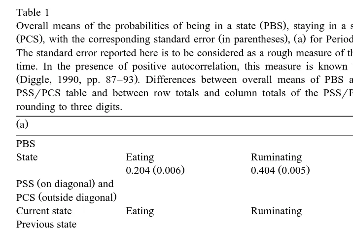
The overall means of the probabilities PBS Table 1 show that on average across a day, the likelihood of a sheep eating was equal to about half the likelihood of it being ruminating or idling. Differences between Periods 1 and 4 in the PBS overall means were of moderate importance, with decreases of 0.017 for eating and of 0.006 for ruminating, and an increase of 0.023 for idling. Differences between PBS and PSS
Table 1
Ž . Ž .
Overall means of the probabilities of being in a state PBS , staying in a state PSS and changing of state
ŽPCS , with the corresponding standard error in parentheses , a for Period 1 and b for Period 4. Ž . Ž . Ž .
The standard error reported here is to be considered as a rough measure of the variability of probabilities over time. In the presence of positive autocorrelation, this measure is known to suffer from a downward bias
ŽDiggle, 1990, pp. 87–93 . Differences between overall means of PBS and row or column totals of the.
PSSrPCS table and between row totals and column totals of the PSSrPCS table are due mainly to the rounding to three digits.
Eating 0.193 0.005 -0.001 -0.001 0.011 0.001
Ž . Ž . Ž .
Ruminating 0.001 -0.001 0.385 0.004 0.018 0.001
Ž . Ž . Ž .
Idling 0.009 -0.001 0.017 0.001 0.366 0.004
Ž .b
Eating 0.174 0.005 0.001 -0.001 0.012 0.001
Ž . Ž . Ž .
Ruminating 0.001 -0.001 0.374 0.004 0.024 0.001
Ž . Ž . Ž .
Ž .
overall means did not exceed 0.034 i.e., for idling in Period 4 ; this result followed from our choice of the minute as sampling time interval and the proportion of acts shorter than 1 min. Accordingly, differences between periods in the overall means of PSS were similar to those in the overall means of PBS. Overall mean values of the probabilities of changing of state were much lower than those of staying in the same state. In decreasing order of likelihood were the transitions: ruminating™idling and the converse, eating™idling and the converse, and eating™ruminating and the converse. In particular, transitions involving eating and ruminating were very rare. The largest differences between periods in the overall means of PCS were observed for the transition ruminating™ idling and its converse, which were more frequent in Period 4 than in Period 1.
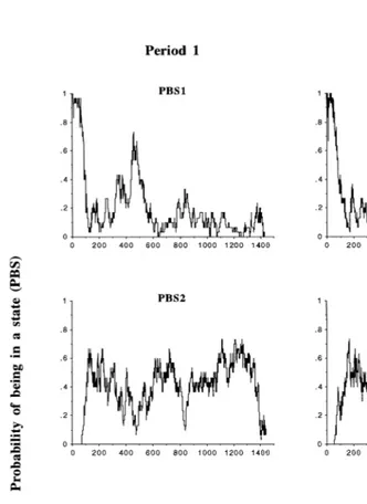
In view of Fig. 2, the following preliminary observations can be made on the mean series of the PBS probabilities.
Ž .1 As it might be expected, the likelihood of the eating state i.e., PBS1 presentedŽ .
two main peaks about 0 and 420 min after the first feeding of the day. Obviously, these peaks corresponded to the two feedings at 0900 and 1600 h and the two main meals of the sheep.
Ž .2 However, whereas all animals were eating at 0900 h on all days without
exception, such unanimity was not observed at 1600 h, as some of the animals were
Ž
ruminating or idling at that time on some days in each period see the PBS2 and PBS3
.
mean series .
More interestingly, a number of differences between Periods 1 and 4 may be
Ž .
observed on the mean series of PBS1 Fig. 2 .
Ž3.1 The major difference concerns the presence of a secondary peak in PBS1 about.
Ž .
330–375 min after the first feeding i.e., between 1430 and 1515 h in Period 1, whereas such a peak was totally absent in Period 4. That secondary peak in PBS1 in Period 1 fell
Ž .
within a wider time interval i.e., from 325 to 525 min after the first feeding , over which the likelihood of the eating state was continuously above 0.2 and to which belonged the main peak of the second feeding. At the same time of day in Period 4, the likelihood of the eating state was above 0.2 only from 420 to 480 min after the first feeding, due to a sharper peak after 1600 h and no secondary peak between 1430 and 1515 h. Actually, there were mainly two times of day during which the sheep were
Ž .
engaged in eating in Period 4 i.e., from 0900 to 1100 h and between 1600 and 1700 h
Ž .
and both of them directly followed the presentation of a stimulus i.e., the feeding .
Ž3.2 A secondary peak of lesser importance was observed in PBS1 in Period 1, about.
Ž .
840 min after the first feeding i.e., around 2300 h . A similar peak was present in PBS1
Ž .
in Period 4, but about 2 h earlier i.e., 720 min after the first feeding . This result might be related to photoperiod effects, although the difference in daylength between Periods 1 and 4 was only of 60 min. Similarly, photoperiod effects may be put forward for the
Ž
difference observed in PBS1 after the second feeding of the day i.e., from 480 to 525
.
min after the first feeding .
Ž3.3 A sharp decrease in PBS1, from 1.0 to about 0.67, was observed a few minutes.
after the first feeding in Period 4. It corresponded to a simultaneous increase in the
Ž .
Fig. 2. Mean series of time-dependent probabilities of being in each of the three chewing behavioural states in Periods 1 and 4. State 1seating; state 2sruminating; state 3sidling; for example, PBS1sprobability of
Ž .
The observations to be made on the mean series of PBS2 and PBS3 in Fig. 2 are less numerous than for PBS1. Differences between periods in PBS2 and PBS3 are also less noticeable.
Ž .4 In both periods, the likelihood of the ruminating state i.e., PBS2 was 0.0 at theŽ .
time of first feeding and remained 0.0 for about an hour, before reaching a value of 0.65–0.75 after 120–180 min and fluctuating around 0.5 thereafter. Troughs in PBS2
Že.g., at the time of second feeding corresponded to peaks in PBS1..
Ž .5 The main differences between periods in PBS2 were characterised by a smooth decrease from 0.5 to 0.07 in the 5–8 h following the first feeding and a pronounced trough about 840 min after the first feeding in Period 1, compared to a sharper decrease and a lagged trough of lesser importance in Period 4. These differences coincided with the differences reported for PBS1.
Ž .6 The mean series of PBS3 showed similarities with those of PBS2. In both periods,
the mean series of PBS3 started at 0.0 and remained low for about an hour, before reaching a value of about 0.5 after 100–120 min and maintaining stable around 0.4
Ž
thereafter. By contrast, in the last minutes before the first feeding of the next day i.e.,
.
while the individual pens of the sheep were cleaned , the animals were mostly idling.
Ž .7 The main difference between periods in PBS3 was the presence of a pronounced
Ž .
trough around 0400 h i.e., 1140 min after the first feeding in Period 1 and the absence of such a peak in Period 4. That trough in PBS3 in Period 1 corresponded to a peak in PBS2 at the same time.
Ž .
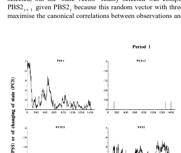
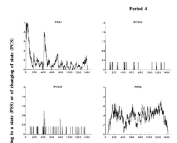
Overall, the temporal pattern of the PSS mean series see diagonals in Fig. 3 was
Ž .
similar to that of the PBS mean series Fig. 2 . This result followed from our choice of the minute as sampling interval and the proportion of acts shorter than 1 min. The
Ž
clearest differences between PSS and PBS mean series were observed for idling i.e., the
.
state with the highest proportion of acts shorter than 1 min , but these differences remained minor. Accordingly, we do not discuss the PSS mean series any further. Instead, we focus on the PCS mean series. These reproduced the majority of changes of state because of the 1-min sampling interval. If we had used a 5-min sampling interval, we would have missed most of the transitions involving the idling state, for which the
Ž .
frequency of acts shorter than 5 min was predominant i.e., )50% . The temporal distribution of transitions was very different, depending on the pair of states involved: the transition eating™ruminating and its converse were very sparse, especially in Period 1, and showed no real pattern; the transition eating™idling and its converse
Ž .
were concentrated around the times of feeding and the peaks in PBS1 Fig. 2 ; the transition ruminating™idling and its converse were more uniformly distributed over the day, with troughs at the times of feeding and fluctuations elsewhere. Overall, the PCS mean series of a given transition tended to have a temporal pattern similar to that of the converse. The main difference between periods in the PCS mean series was observed for PCS13 and PCS31, which showed higher peaks in Period 4 than in Period 1. This result is in accordance with the overall means of PCS13 and PCS31 reported in Table 1.
All three mean series of PBS1, PBS2 and PBS3 were strongly and positively autocorrelated. This result indicates that high values generally succeeded to high values
Ž .
in Period 1 and 0.96 in Period 4 for PBS2, and 0.95 in Period 1 and 0.94 in Period 4 for
Ž .
PBS3. Restricting autocorrelation analysis to the first half of the series i.e., ns720 provided similar results. For recall, only two of the three PBS mean series could be used in state-space modelling. On the basis of the autocorrelation analysis results above, it was justified to use PBS1 and PBS2 because their mean series were more positively
Ž .
autocorrelated, which would facilitate forecasting Box et al., 1994 . The cross-correla-tions between PBS1 and PBS2 were weaker than their respective autocorrelacross-correla-tions and negative, indicating that peaks in PBS1 tended to correspond to troughs in PBS2, and reversely. For each of the two periods, a second-order autoregressive model was selected, but the ‘state vector’ finally selected was composed of PBS1 , PBS2 andt t PBS2tq1 given PBS2 because this random vector with three components was found tot maximise the canonical correlations between observations and forecasts. Using that state
Ž .
Fig. 3. Mean series of time-dependent probabilities of staying in a state diagonal panels and changing of state
Žoff-diagonal panels in Periods 1 and 4. State 1. seating; state 2sruminating; state 3sidling; for example, PSS1sprobability of staying in state 1 and PCS12sprobability of transition from state 1 to state 2. The
Ž .
Ž .
Fig. 3 continued .
vector, the state-space model was fitted to the mean series of PBS1 and PBS2 over ts0, . . . , 719. Thereafter, forecasts of PBS1-3 were obtained for a maximum lead of
Ž . 2
720 min i.e., ts720, . . . , 1439 and the coefficient of determination R was calculated between observations and forecasts.
Not surprisingly, forecasts of PBS1-3 were not reliable for the lead of 720 min. However, in Period 1, forecasts differed from observations by less than 0.1 up to a lead of 37 min for eating, 23 min for ruminating and 43 min for idling; the R2 values
calculated for these leads were 0.145, 0.625, and 0.573, respectively. Thus, the quality of forecasts tended to depend on the type of acts in Period 1: acts in which the sheep
Ž .
spent less energy i.e., idling appeared to be predictable at longer term, whereas acts in
Ž .
which the sheep spent the most energy i.e., eating were the most difficult to forecast accurately. Things were different in Period 4. In this period, differences between observations and forecasts were smaller than 0.1 up to a lead of 23 min for eating, 25 min for ruminating and 23 min for idling; the R2 values were 0.049, 0.484, and 0.232,
Ž .
an effect on the quality of forecasts because it was high i.e.,G0.94 for all PBS mean series in both periods, as ensured by the 1-min sampling interval used in the calculation of time-dependent transition probabilities. These results support Hypothesis I to some extent: the quality of forecasts decreased from Period 1 to Period 4, and the ranking of states with regard to the quality of forecasts changed on the basis of leads of reliable forecasts, but not on the basis of R2 values.
Eating, more than the two other chewing behavioural states, showed significant differences between periods in the ANOVA of the finite Fourier transform. For this state, the absence of period effects was rejected at the 0.05 level at four of the 24 first Fourier frequencies: frequency 1, which corresponds to the fundamental component of the nycterohemeral rhythm and is represented by a trigonometric function cycling every 24 h, and frequencies 10, 14, and 24, which are high-order harmonics of the former and correspond to cycles of 2.4, 1.7, and 1 h. By comparison, only one significant difference between periods was observed for ruminating, at Fourier frequency 14, and another one
Ž .
for idling, at frequency 7; this rejection rate i.e., 1r24s0.04 was even less than the theoretical significance level of 0.05 that was used in statistical testing. Accordingly, we focused on the eating state in our post-hoc spectral analyses.
The significant period effects at four Fourier frequencies for eating were charac-terised by differences in the periodogram ordinates calculated from the PBS1 mean series and by phase delays calculated as Period 4 phase minus Period 1 phase. Periodogram ordinates were 11.00, 2.71, 0.80, 0.23 in Period 1 vs. 9.73, 1.69, 1.85, 0.65 in Period 4 at frequencies 1, 10, 14, and 24, respectively. The corresponding phase delays were 66.29, 17.11, 20.02, and 7.22 min. The differences in periodogram ordinates
Ž .
indicate that the lower frequency components i.e., 1, 10 had a larger amplitude in Period 1 than in Period 4, whereas the reverse was true for the higher frequency
Ž .
components i.e., 14, 24 . The fact that the phase delays were systematically positive at the four frequencies shows that the corresponding frequency components reached their peak earlier in Period 4 than in Period 1, as a possible effect of the shorter daylength in Period 4. These results support Hypothesis II for eating, but not for ruminating and idling.
3.3. Age-dependent model
General patterns displayed in Fig. 4 are the increase of transition probabilities with age when the two transition states are different and the decrease of transition probabili-ties with age when the two states are the same. The strange pattern of the age-dependent model for the transition eating™ruminating and its converse is due to the scarcity of these transitions in our experiment.
Ž .
Over the whole range of ages considered i.e., 1–60 min , the relationship between
Ž .
transition probability and age is curvilinear instead of linear Fig. 4 . However, both at
Ž . Ž .
small scale 1–6 min and at small-to-intermediate scale 5–20 min , the linearity of the relationship seems almost perfect. With the exceptions of the transition eating™ ruminating and its converse, minor differences between periods are observed in Fig. 4. The two last points were investigated further by fitting separate simple linear
Ž .
regressions on age over the 1–6 min range small scale and over the 5–20 min range
Žsmall-to-intermediate scale . The intercept and slope of the fitted models varied.
Ž .
noticeably with scale for all transitions without exception Table 2 . On the other hand,
Ž 2 .
all the age-dependent models were almost purely linear at each scale i.e., R ;1.0 , with the two exceptions mentioned above. Besides the rare transitions, the most important differences between periods were observed for the transitions eating™eating, ruminating™ruminating, and idling™ruminating. These differences were more in the intercept, with constant discrepancies with increasing age, than in the slope, the rate of decrease or increase of the three transition probabilities being almost identical in the two periods.
3.4. Mean hourly times
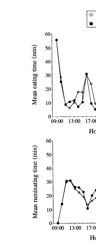
The mean hourly times plotted in Fig. 5 display, to some degree, a number of features of the mean series of probabilities PBS calculated every minute and plotted in Fig. 2.
Table 2
Simple linear regression analyses of age-dependent transition probabilities on age at small scale and at
Ž . Ž .
small-to-intermediate scale a for Period 1 and b for Period 4
a b
Transition Small scale Small-to-intermediate scale
2 2
Fitted model R Fitted model R
( )a
Eating™eating 0.201y0.009 age 0.999 0.182y0.006 age 0.991
Eating™ruminating 0.00006q0.00006 age 0.916 0.0001q0.00003 age 0.580
Eating™idling 0.004q0.008 age 0.995 0.022q0.005 age 0.991
Ruminating™eating 0.00001q0.001 age 0.999 0.001q0.0004 age 0.991 Ruminating™ruminating 0.398y0.015 age 0.999 0.374y0.011 age 0.993 Ruminating™idling 0.006q0.014 age 0.997 0.025q0.011 age 0.997
Idling™eating 0.006q0.004 age 0.986 0.017q0.002 age 0.990
Idling™ruminating 0.009q0.010 age 0.994 0.027q0.007 age 0.994
Idling™idling 0.377y0.014 age 0.987 0.351y0.010 age 0.997
( )b
Eating™eating 0.182y0.009 age 0.997 0.154y0.005 age 0.975
Eating™ruminating 0.00003q0.0005 age 0.998 0.0003q0.0004 age 0.909
Eating™idling 0.005q0.009 age 0.994 0.029q0.005 age 0.976
Ruminating™eating 0.0002q0.001 age 0.992 0.003q0.001 age 0.891 Ruminating™ruminating 0.387y0.016 age 0.994 0.362y0.012 age 0.996 Ruminating™idling 0.011q0.015 age 0.996 0.033q0.011 age 0.995
Idling™eating 0.007q0.004 age 0.988 0.018q0.002 age 0.975
Idling™ruminating 0.014q0.012 age 0.990 0.039q0.008 age 0.994
Idling™idling 0.394y0.016 age 0.991 0.362y0.010 age 0.993
a
Ages1, 2, 3, 4, 5, 6 min.
b
Ž . Ž . Ž . Ž y1.
Fig. 5. Mean hourly time spent A eating, B ruminating, and C idling min h in Periods 1 and 4.
Ž
Fig. 5, for obvious reasons related to the different sampling intervals i.e., 1 h vs. 1
.
min . Therefore, a number of differences might be expected between the results of the spectral analyses of the PBS mean series and those of mean hourly times.
In fact, the ANOVA of the finite Fourier transform of mean hourly times, with period
Ž .
as classification factor, provided: 1 significant period effects at two of the 12 Fourier
Ž . Ž . Ž .
frequencies, frequency 1 like PBS1 and frequency 6 unlike PBS1 , for eating; 2 no
Ž .
significant period effect at any Fourier frequency for ruminating; 3 one significant
Ž .
period effect at Fourier frequency 7 for idling like PBS3 . The significant period effects observed for the mean hourly time spent eating were characterised by an important difference in the periodogram ordinates at the fundamental nycterohemeral frequency
Ži.e., 673.1 for Period 1 vs. 591.1 for Period 4 and by a phase delay of about 3.5 h at.
frequency 6. With the exceptions of frequency 1 for eating and frequency 7 for idling, the frequencies at which significant period effects were detected for mean hourly times were all lower than for the corresponding probabilities PBS. As mentioned above, the explanation is to be found in the smoothing of data that resulted from the use of hourly times. Moreover, in spectral analysis, the use of a sampling interval longer than suited is known to result in an ‘aliasing effect’, that is, rhythmic components that are supposed to
Ž .
be detected at high frequencies e.g., frequencies 19, 24 in PBS1 are out of range if the sampling interval is too long, and such rhythmic components then erroneously appear at
Ž .
lower frequencies Priestley, 1981 . An ANOVA of the periodogram ordinates alone
Ži.e., the ANOVA of the finite Fourier transform combines amplitudes and phases in the .
same analysis; Deswysen et al., 1989 did not avoid the problem, neither did smoothing the periodogram by a triangular spectral window.
4. Discussion
Seasonal effects on voluntary food intake and growth have long been studied in
Ž
sheep, through photoperiod and temperature Hoersch et al., 1961; Gordon, 1964; see
.
Arnold, 1981, 1985 for a general review . Differences in the experimental conditions, the collection of data and their quantitative analysis do not facilitate direct comparison
Ž
of results of the literature with our own results. Many factors e.g., housing vs. stocking
.
on pasture, physiological status, age, breed, diet are involved in the reported studies and it is understood that the results summarised below have been observed in the specific conditions of each study that we refer to. Moreover, the ingestive behaviour has generally been studied on a daily basis, and when it was studied within a day, the overall
Ž .
period of time was limited e.g., 1 week because the objective was not the investigation
Ž .
of seasonal effects Champion et al., 1994 .
There is some evidence in the literature for temperature effects on the voluntary food intake and growth of domestic animals. However, the most significant temperature effects were observed for extreme temperature regimes, such as maximum temperatures
Ž .
of y24 to q58C in cattle Malechek and Smith, 1976 and a constant temperature of
Ž . Ž .
32.28C in sheep Hoersch et al., 1961 . Note that Hoersch et al. 1961 found an effect of temperature on growth rate, but not on feed consumption. Since the mean
tempera-Ž .
our study, the differences between periods that we found in the eating state of chewing behaviour are not likely to be due to temperature. As the sheep were continuously
Ž .
wooled, any cold stress following the shearing of sheep Arnold and Birrell, 1977 cannot be suggested either.
By maintaining temperature and humidity constant, Michalet-Doreau and Gatel
Ž1988 pointed out photoperiod effects on the daily hay intake by sheep. These effects.
are of sinusoidal type over the year, with the minimum intake occurring in the first half
Ž
of February and the maximum in the first half of August i.e., 45 days after the winter
.
and summer solstices . The differences between Periods 1 and 4 that we found in PBS1 are in accordance with the acknowledgment that the voluntary food intake of sheep is
Ž .
higher in summer than in winter Iason et al., 1995 . In general, differences in voluntary food intake between summer and winter are attributed to the daylength or photoperiod
Že.g., Foot and Russel, 1978; Forbes et al., 1979; Schanbacher and Crouse, 1980 . The.
secondary peaks in PBS1 that we observed later in the evening in Period 1 than in
Ž .
Period 4 Fig. 2 and the phase delays in our post-hoc spectral analyses confirm those results. To the best of our knowledge, no seasonal effects on the ruminating and idling states of chewing have ever been reported in the literature, and those that we reported here for sheep were minor, compared to eating.
Ž .
The results reported by Rook and Penning 1991 on the grazing behaviour of sheep allow a more direct comparison with our results, even if the data analysed by Rook and
Ž .
Penning 1991 came from an experiment covering the period of October to July and the
Ž .
sheep were not housed but stocked on pasture Penning et al., 1991 . In fact, the probabilities reported here in Table 1 are referred to as the probabilities calculated under
Ž
the ‘multinomial model’ and the ‘Markov model’ by Rook and Penning 1991, Tables 1
.
and 2 , that is, under the independence and the Markovian assumption, respectively. The differences between their study and ours with regard to these probabilities are substantial
Ž
and are to be attributed to differences in the experimental conditions i.e., grazing
.
animals are known to spend more time eating; Arnold, 1985 and in the sampling
Ž .
interval i.e., 1 min here vs. 5 min in Rook and Penning, 1991 .
The development of appropriate statistical methods for an effective analysis of behavioural data is motivating quantitative ethologists in their research work for decades
ŽCane, 1959; Wiepkema, 1961; Nelson, 1964; Delius, 1969; Altmann, 1974 . Following.
the QuantitatiÕe Methods in Ethology and QuantitatiÕe Methods in BehaÕior symposia
Ž .
held middle of the 70s Hazlett, 1977; Colgan, 1978 , it was established that judicious quantification had become an essential aspect of the ethological approach to behaviour
ŽDunham, 1978 . Graphical methods, autocorrelation and spectral analyses, and straight-.
forward hypothesis testing techniques were presented, among others, as indicated methods for the analysis of behavioural data; the modelling approach was also strongly
Ž .
supported Fagen and Young, 1978 . The future was announced to belong to those who could use simple methods effectively to test a theoretical hypothesis or could construct original models of behaviour, should no simple technique be available. Since the middle of the 70’s, a number of models and methods that relax the Markovian and stationarity
Ž
assumptions to various degrees and ‘allow memory to operate’ have been proposed e.g.,
.
provide to the problems of temporal dependency and non-stationarity remain specific, and once the transition probabilities are calculated, the graphical or quantitative aspects of these methods are limited. Thus, the method of time-dependent transition probabilities introduced here represents a complement to them. The new method applies whenever animals are followed individually and their behaviour is recorded continuously, simulta-neously and repeatedly over time.
Ž .
The results that we obtained using the age-dependent model Table 2 and Fig. 4 , and especially the increase with age of the transition probabilities involving two different
Ž .
states, are in agreement with Rook and Penning’s 1991 intuition that an animal should be more likely to cease a particular activity if it has been engaged in that activity for a long time. The authors also put forward some intake control theories to support their statement, and our results confirm theirs. On the other hand, the transition probabilities calculated under the age-dependent model do not compare directly with the probabilities PCS. The former are calculated for different ‘ages’ and indicate how the transition probabilities increase or decrease as functions of the time elapsed since the animal is engaged in a given activity. The probabilities PCS are functions of the time elapsed from
Ž .
a reference point e.g., the first feeding of the day in our study and indicate the times of day at which changes of state are more, or less, likely to occur, using a sampling interval that avoids redundancy and ensures sufficiency. In our study, the time-dependent transition probabilities, and PBS1 in particular, elucidated the question of the time of day during which the sheep ate less in Period 4 than in Period 1, that is, from where
Ž .
comes the decrease in voluntary food intake observed by Despres 1993 .
`
5. Conclusions
The most significant seasonal effects on within-day variations in the chewing behaviour of housed sheep have been observed for eating in this study. In particular, the nycterohemeral pattern of the eating state is more affected than those of ruminating and
Ž .
Acknowledgements
This work was supported by The Natural Sciences and Engineering Research Council
Ž .
of Canada NSERC and Le Fonds pour la Formation de Chercheurs et l’Aide a la
`
Ž .
Recherche du Quebec FCAR , through research grants to the senior author. The second
´
author acknowledges a NATO fellowship during his sabbatical leave in Canada. We are grateful to L. Despres and E. Amouche for their contribution to the experiment from
`
which originate the data analysed in this paper. We benefited from the computing facilities of McGill University for the statistical analyses of the data. We are grateful to two anonymous reviewers for their comments on an earlier version of the manuscript.
References
Akaike, H., 1974. Markovian representation of stochastic processes and its application to the analysis of autoregressive moving average processes. Ann. Inst. Stat. Math. 26, 363–387.
Akaike, H., 1976. Canonical correlation analysis of time series and the use of information criterion. In: Mehra,
Ž .
R., Lainiotis, D.G. Eds. , Advances and Case Studies of System Identification. Academic Press, New York, pp. 27–96.
Altmann, J., 1974. Observational study of behaviour: sampling methods. Behaviour 49, 227–267.
Ž .
Arnold, G.W., 1981. Grazing behaviour. In: Morley, F.H.W. Ed. , World Animal Science, B.I. Grazing Animals. Elsevier, Amsterdam, pp. 79–104.
Ž .
Arnold, G.W., 1985. Ingestive behaviour. In: Fraser, A.F. Ed. , Ethology of Farm Animals. Elsevier, Amsterdam, pp. 183–200.
Arnold, G.W., Birrell, H., 1977. Food intake and grazing behaviour of sheep varying in body condition. Anim. Prod. 24, 343–353.
Arnold, G.W., Dudzinski, M.L., 1978. The Ethology of Free-ranging Domestic Animals. Elsevier, Amsterdam, 198 pp.
Box, G.E.P., Jenkins, G.M., Reinsel, G.C., 1994. Time Series: Forecasting and Control. 3rd edn. Prentice-Hall, Englewood Cliffs, pp. 598.
Brillinger, D.R., 1973. The analysis of time series collected in an experimental design. In: Krishnaiah, P.R.
ŽEd. , Multivariate Analysis III. Academic Press, New York, pp. 241–256..
Ž .
Brillinger, D.R., 1980. Analysis of variance and problems under time series models. In: Krishnaiah, P.R. Ed. , Handbook of Statistics 1: Analysis of Variance. North-Holland, Amsterdam, pp. 237–278.
Brownie, C., Hines, J.E., Nichols, J.D., Pollock, K.H., Hestbeck, J.B., 1993. Capture–recapture studies for multiple strata including non-Markovian transitions. Biometrics 49, 1173–1187.
Cane, V., 1959. Behaviour sequences as semi-Markov chains. J. R. Stat. Soc. B 21, 36–58.
Champion, R.A., Rutter, S.M., Penning, P.D., Rook, A.J., 1994. Temporal variation in grazing behaviour of sheep and the reliability of sampling periods. Appl. Anim. Behav. Sci. 42, 99–108.
Colgan, P.W., 1978. Quantitative Ethology. Wiley, New York, pp. 364.
Delius, J.D., 1969. A stochastic analysis of the maintenance behaviour of skylarks. Behaviour 33, 137–178.
´
Despres, L., 1993. Etude de la repetabilite des mesures de quantites ingerees de digestibilite et du` ´ ´ ´ ´ ´ ´ ´
Ž
comportement alimentaire et merycique chez des ovins en stabulation. Memoire de fin d’etudes Ingenieur´ ´ ´ ´
.
agronome , Universite catholique de Louvain.´
Deswysen, A.G., Dutilleul, P., Ellis, W.C., 1989. Quantitative analysis of nycterohemeral eating and ruminating patterns in heifers with different voluntary intakes and effects of monensin. J. Anim. Sci. 67, 2751–2761.
Dudzinski, M.L., Arnold, G.W., 1979. Factors influencing the grazing behaviour of sheep in a Mediterranean environment in summer. Appl. Anim. Ethol. 5, 125–144.
Ž .
Dunham, D.W., 1978. Foreword. In: Colgan, P.W. Ed. , Quantitative Ethology. Wiley, New York, pp. vii–viii.
Dutilleul, P., 1990. Apport en analyse spectrale d’un periodogramme modifie et modelisation des series´ ´ ´ ´
chronologiques avec repetitions en vue de leur comparaison en frequence. Doctoral dissertation, Universite´ ´ ´ ´
catholique de Louvain.
Dutilleul, P., 1998. Incorporating scale in ecological experiments: data analysis. In: Peterson, D.L., Parker,
Ž .
V.T. Eds. , Ecological Scale: Theory and Applications. Columbia Univ. Press, New York, pp. 387–425. Dwyer, D.D., 1991. Activities and grazing preferences of cows with calves in northern Osage Country, OK.
Bull. Okla. Agric. Exp. Stn., No. B-588, pp. 61.
Fagen, R.M., Young, D.Y., 1978. Temporal patterns of behaviors: durations, intervals, latencies, and
Ž .
sequences. In: Colgan, P.W. Ed. , Quantitative Ethology. Wiley, New York, pp. 79–114.
Foot, J.Z., Russel, J.F., 1978. Pattern of intake of three roughage diets by non-pregnant, non-lactating Scottish Blackface ewes over a long period and the effects of previous nutritional history on current intake. Anim. Prod. 26, 203–215.
Forbes, J.M., El Shahat, A.A., Jones, R., Duncan, J.G.S., Boaz, T.G., 1979. The effect of daylength on the growth of lambs: 1. Comparisons of sex, level of feeding, shearing, and breed of sire. Anim. Prod. 29, 33–42.
Gordon, J.G., 1964. Effect of time of year on the roughage intake of housed sheep. Nature 204, 798–799. Hazlett, B.A., 1977. Quantitative Methods in the Study of Animal Behaviour. Academic Press, New York,
pp. 222.
Hoersch, T.M., Reineke, E.P., Henneman, H.A., 1961. Effect of artificial light and ambient temperature on the thyroid secretion rate and other metabolic measures in sheep. J. Anim. Sci. 20, 358–362.
Hurnik, J.F., Mullen, K., 1981. Detection of a change in frequency of behavioural activity. Appl. Anim. Ethol. 7, 287–292.
Iason, G.R., Sim, D.A., Foreman, E., 1995. Seasonal changes in intake and digestion of chopped timothy hay
ŽPhleum pratense by three breeds of sheep. J. Agric. Sci. 125, 273–280..
Jones, R.H., 1993. Longitudinal Data with Serial Correlation: A State-space Approach. Chapman & Hall, London, pp. 225.
Low, W.A., Tweedie, R.L., Edwards, C.H.B., Hodder, R.M., Malafant, K.W.J., Cunningham, R.B., 1981. The influence of environment on daily maintenance behaviour of free ranging shorthorn cows in Central Australia: I. General introduction and descriptive analysis of day-long activities. Appl. Anim. Ethol. 7, 11–26.
Malechek, J.C., Smith, E.M., 1976. Behaviour of range cows in response to winter weather. J. Range Manage. 29, 9–12.
´
Michalet-Doreau, B., Gatel, F., 1988. Evolution au cours d’une annee des quantites de foin ingerees par des´ ´ ´ ´
beliers castres. Ann. Zootech. 37, 151–158.´ ´
Ž
Nelson, K., 1964. The temporal patterning of courtship behavior in the glandulocaudine fishes Ostariophysi,
.
Characidae . Behaviour 24, 90–146.
Ž .
Oden, N., 1977. Partitioning dependence in nonstationary behavioural sequences. In: Hazlett, B.A. Ed. , Quantitative Methods in the Study of Animal Behaviour. Academic Press, New York, pp. 203–220. Penning, P.D., Parsons, A.J., Orr, R.J., Harvey, A., Champion, R.A., 1995. Intake and behaviour responses by
sheep, in different physiological states, when grazing monocultures of grass or white clover. Appl. Anim. Behav. Sci. 45, 63–78.
Penning, P.D., Rook, A.J., Orr, R.J., 1991. Patterns of ingestive behaviour of sheep continuously stocked on monocultures of ryegrass or white clover. Appl. Anim. Behav. Sci. 31, 237–250.
Priestley, M.B., 1981. Spectral Analysis and Time Series. Academic Press, London, pp. 890.
Rook, A.J., Penning, P.D., 1991. Stochastic models of grazing behaviour in sheep. Appl. Anim. Behav. Sci. 31, 237–250.
Ruckebusch, Y., 1963. Recherches sur la regulation centrale du comportement alimentaire des ruminants.´
Doctoral dissertation, Universite de Lyon.´
SAS Institute, 1988. SASrETSw
User’s Guide, Version 6. SAS Institute, Cary, pp. 560. SAS Institute, 1989. 4th edn. SASrSTATw
Schanbacher, B.D., Crouse, J.D., 1980. Growth and performance of growing-finishing lambs exposed to long or short photoperiods. J. Anim. Sci. 51, 943–948.
Ž .
Slater, P.J.B., 1978. Data collection. In: Colgan, P.W. Ed. , Quantitative Ethology. Wiley, New York, pp. 7–24.
Snedecor, G.W., Cochran, W.G., 1967. Statistical Methods. 6th edn. Iowa State Univ. Press, Ames, pp. 593.
Ž
Wiepkema, P.R., 1961. An ethological analysis of the reproductive behaviour of the bitterling Rhodeus
.