High Resolution FDMA MIMO Radar
David Cohen, Deborah Cohen,
Student IEEE
and Yonina C. Eldar,
Fellow IEEE
Abstract—Traditional multiple input multiple output radars, which transmit orthogonal coded waveforms, suffer from range-azimuth resolution trade-off. In this work, we adopt a frequency division multiple access (FDMA) approach that breaks this conflict. We combine narrow individual bandwidth for high azimuth resolution and large overall total bandwidth for high range resolution. We process all channels jointly to overcome the FDMA range resolution limitation to a single bandwidth, and address range-azimuth coupling using a random array configuration.
I. INTRODUCTION
Multiple input multiple output (MIMO) [1] radar combines several antenna elements both at the transmitter and receiver. Unlike phased-array systems, each transmitter radiates a dif-ferent waveform, which offers more degrees of freedom [2]. Today, MIMO radars appear in many military and civilian applications including ground surveillance [3], [4], automotive radar [5], [6], interferometry [7], maritime surveillance [3], [8], through-the-wall radar imaging for urban sensing [9] and medical imaging [2], [10]. There are two main configurations of MIMO radar, depending on the location of the transmitting and receiving elements; collocated MIMO [11] in which the elements are close to each other relatively to the working wavelength, and multistatic MIMO [12] where they are widely separated. In this work, we focus on collocated MIMO sys-tems.
MIMO radar presents significant potential for advancing state-of-the-art modern radar in terms of flexibility and perfor-mance. Collocated MIMO radar systems exploit the waveform diversity, based on mutual orthogonality of the transmitted signals [2]. Consequently, the performance of MIMO systems can be characterized by a virtual array corresponding to the convolution of the transmit and receive antenna locations. In principle, with the same number of antenna elements, this virtual array may be much larger and thus achieve higher reso-lution than an equivalent traditional phased array system [13], [14], [15].
The orthogonality requirement, however, poses new theo-retical and practical challenges. Choosing proper waveforms is a critical task for the implementation of practical MIMO radar systems. In addition to the general requirements on radar waveforms such as high range resolution and low sidelobes, MIMO radar waveforms must satisfy good orthogonality prop-erties. In practice, it is difficult to find waveform families that perfectly satisfy all these demands [16]. Comprehensive evaluation and comparison of different types of MIMO radar waveforms is presented in [17], [18], [19]. The main waveform
This project is funded by the European Union’s Horizon 2020 research and innovation program under grant agreement No. 646804-ERC-COG-BNYQ, and by the Israel Science Foundation under Grant no. 335/14. Deborah Cohen is grateful to the Azrieli Foundation for the award of an Azrieli Fellowship.
families considered are time, frequency and code division multiple access, abbreviated as TDMA, FDMA and CDMA, respectively. These may either be implemented in a single pulse, namely in the fast time domain, referred to as intra-pulse coding or in a intra-pulse train, that is in the slow time domain, corresponding to inter-pulse coding. We focus on the former technique, which is most popular. More details on inter-pulse coding can be found in [17], [19].
An intuitive and simple way to achieve orthogonality is using TDMA, where the transmit antennas are switched from pulse to pulse, so that there is no overlap between two transmissions [20]. Since the transmission capabilities of the antennas are not fully utilized, this approach induces significant loss of transmit power [17], resulting in signal to noise ratio (SNR) decrease and much shorter target detection range. More efficient schemes have been proposed, such as circulating MIMO waveforms [18]. However, this technique suffers from loss in range resolution [18], [19].
Another way to achieve orthogonality of MIMO radar wave-forms is FDMA, where the signals transmitted by different antennas are modulated onto different carrier frequencies. This approach suffers from several limitations. First, due to the linear relationship between the carrier frequency and the index of antenna element, a strong range azimuth coupling occurs when using the classic virtual uniform linear array (ULA) configuration [16], [18], [19]. To resolve this aliasing, the authors in [21] use random carrier frequencies, which creates high sidelobe level. These may be mitigated by increasing the number of transmit antennas, which in turn increases system complexity. The second drawback of FDMA is that the range resolution is limited to a single waveform’s bandwidth, rather than the overall transmit bandwidth [22], [23]. To increase range resolution, the authors of [24], [25] use an inter-pulse stepped frequency waveform (SFW), utilizing the total bandwidth over the slow time [26], [27]. However, SFW leads to range-Doppler coupling [28] and the pulse repetition frequency (PRF) increases proportionally to the number of steps increasing range ambiguities [20], [29].
In the popular CDMA approach, signals transmitted by different antennas are modulated using distinct series of or-thogonal codes, so that they can be separated in the radar receiver. Although perfect orthogonality cannot in general be achieved, code families, such as Barker [30], Hadamard or Walsh [31] and Gold [32] sequences, present features close to orthogonality. CDMA requires good code design [2] and may suffer from high range sidelobes depending on cross-correlation properties of the code sequence [19]. More im-portantly, the narrowband assumption, that ensures constant delays over the channels, creates a trade-off between azimuth and range resolution, which can be a limiting factor for high resolution applications, by requiring either small aperture or
small total bandwidth. In CDMA, the total bandwidth is equal to the individual bandwidth of each waveform, cre-ating a conflict between large desired bandwidth for high range resolution and large virtual aperture for high azimuth resolution [33]. The trade-off comes from the beamforming performance degradation when using wideband signals, since this operation is frequency dependent [34]. This dependency is quite severe in MIMO configurations where the virtual array is large. Several works [35], [36] incorporate filter banks to ensure frequency invariance. However, in doing so, they increase system complexity at the receiver. In [33], a smearing filter is adopted to address system complexity which in turn leads to poor range resolution.
In this work, we adopt the FDMA approach and present an array design and processing method that overcome its draw-backs. First, to avoid range-azimuth coupling, we randomize the transmit and receive locations within the virtual array aperture. The idea of randomized frequencies has been used in single antenna radars [28] that employ SFW, to resolve range-Doppler coupling. There, hopped frequency sequences, namely with randomized steps for increasing the carriers, have been considered. Random arrays have been an object of research since the 1960s [37]. Recently, in [38], the authors adopt random MIMO arrays to reduce the number of elements required for targets’ detection using sub-Nyquist spatial sam-pling principles [39]. Here, we use a random array to deal with the coupling issue while keeping the number of elements as in traditional MIMO. We empirically found that randomizing the antenna locations rather than the frequencies exhibits better performance.
Second, we process the samples from all channels jointly exploiting frequency diversity [40], to overcome the range resolution limitation of a single bandwidth. A similar approach was used in [41] in the context of MIMO synthetic aperture radar (SAR) with orthogonal frequency-division multiplexing linear frequency modulated (OFDM LFM) waveforms, where coherent processing over the channels allows to achieve range resolution corresponding to the total bandwidth. There, how-ever, the MIMO array is composed of two uniform linear arrays (ULAs), both with spacing equal to half the wavelength. While avoiding range-elevation coupling, this approach yields poor elevation resolution [15]. Furthermore, in [41], the total bandwidth is limited by the narrowband assumption [33] and hence perpetuates the range-azimuth resolution conflict. Our approach does not require coding design and allows simpler matched filtering (MF) implementation than CDMA.
The main contribution of this work is to show that using FDMA, the narrowband assumption may be relaxed to the in-dividual bandwidth with appropriate signal processing. FDMA allows us to achieve a large overall received bandwidth over the channels while maintaining the narrowband assumption for each channel. This approach is inspired by SFW, first proposed in single antenna radars, in which a large overall bandwidth is achieved over the slow time to attain high range resolution while maintaining narrow instantaneous bandwidth. The range-azimuth resolution conflict may thus be solved by enabling large aperture for high azimuth resolution along with large total bandwidth for high range resolution. The
narrowband assumption holds by requiring small individual bandwidth, breaking the traditional range-azimuth trade-off. In order to achieve range resolution corresponding to the overall bandwidth, we develop a recovery method that coherently processes all channels. This overcomes the traditional FDMA range resolution limitation to a single bandwidth.
We note that the radar cross section (RCS) may vary with frequency for distributed targets. This is beneficial in extended target applications, where orthogonal frequency division mul-tiplexing (OFDM) may be used for additional frequency diversity as different scattering centers of a target resonate at different frequencies [42]. Unfortunately, when using coherent processing, the reflections from scatterers may interfere con-structively or decon-structively depending on the signal frequency and the phases of the RCS for the individual scatterers [43], [44]. In this work, we adopt the point-target assumption and perform coherent processing. Extended targets can then be modeled as the sum of point scatterers and high resolution may alleviate the above phenomena by separating the point scatterers over some resolution bins [45].
This paper is organized as follows. In Section II, we review classic MIMO pulse-Doppler radar and processing. Our FDMA model is introduced in Section III, where range-azimuth coupling and beamforming are discussed. Section IV presents the proposed range-azimuth-Doppler recovery. Nu-merical experiments are presented in Section V, demonstrat-ing the improved performance of our FDMA approach over classical CDMA.
II. CLASSICMIMO RADAR
We begin by describing the classic MIMO radar archi-tecture, in terms of array structure and waveforms, and the corresponding processing.
A. MIMO Architecture
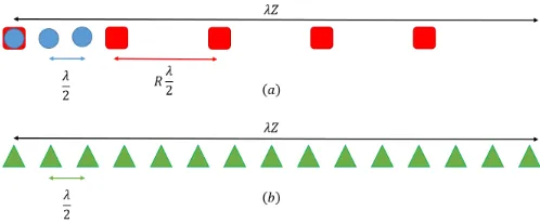
The traditional approach to collocated MIMO adopts a vir-tual ULA structure [46], whereR receivers, spaced by λ2 and
T transmitters, spaced byRλ
Fig. 1. Illustration of MIMO arrays: (a) standard array, (b) corresponding receiver virtual array.
Each transmitting antenna sendsP pulses, such that themth transmitted signal is given by
sm(t) = bandwidth Bh and modulated with carrier frequencyfc. The coherent processing interval (CPI) is equal to P τ, where τ
denotes the pulse repetition interval (PRI). For convenience, we assume that fcτ is an integer, so that the initial phase for every pulse e−j2πfcτ p is canceled in the modulation for
0≤p≤P−1[47]. The pulse time support is denoted byTp, with0< Tp< τ.
MIMO radar architectures impose several requirements on the transmitted waveform family. Besides traditional demands from radar waveforms such as low sidelobes, MIMO transmit antennas rely on orthogonal waveforms. In addition, to avoid cross talk between the T signals and form T R channels, the orthogonality condition should be invariant to time shifts, that is R∞
−∞si(t)s ∗
j(t−τ0)dt = δ(i−j), for i, j ∈ [0, T−1] and for allτ0. This property implies that the orthogonal signals cannot overlap in frequency (or time) [33], leading to the FDMA (or TDMA) approach. Alternatively, time invariant orthogonality can be approximately achieved using CDMA.
Both FDMA and CDMA follow the general model [48]:
hm(t) = Nc
X
u=1
wmuej2πfmutv(t−uδt), (2)
where each pulse is decomposed into Nc time slots with duration δt. Here, v(t) denotes the elementary waveform,
wmu represents the code and fmu the frequency for themth transmission and uth time slot. The general expression (2) allows to analyze at the same time different waveform families. In particular, in CDMA, orthogonality is achieved by the code
{wmu}Nu=1c and fmu = 0 for all 1 ≤ u ≤ Nc. In FDMA,
Nc = 1, wmu = 1 and δt = 0. The center frequencies
fmu = fm are chosen in [−T B2h,T B2h] so that the intervals
[fm−B2h, fm+B2h]do not overlap. For simplicity of notation,
{hm(t)}Tm=0−1 can be considered as frequency-shifted versions of a low-pass pulse v(t) = h0(t) whose Fourier transform
H0(ω)has bandwidthBh, such that
Hm(ω) =H0(ω−2πfm). (3)
We adopt a unified notation for the total bandwidth Btot =
T Bh for FDMA andBtot=Bh for CDMA.
Consider L non-fluctuating point-targets, according to the Swerling-0 model [43]. Each target is identified by its pa-rameters: radar cross section (RCS)α˜l, distance between the target and the array origin or rangeRl, velocityvland azimuth angle relative to the arrayθl. Our goal is to recover the targets’ delay τl = 2Rcl, azimuth sine ϑl= sin(θl)and Doppler shift
fD
l = 2vclfc from the received signals. In the sequel, we use the terms range and delay interchangeably, as well as azimuth angle and sine, and velocity and Doppler frequency.
B. Received Signal
The transmitted pulses are reflected by the targets and collected at the receive antennas. The following assumptions are adopted on the array structure and targets’ location and motion, leading to a simplified expression for the received signal.
A1 Collocated array - target RCSα˜landθlare constant over the array (see [49] for more details).
A2 Far targets - target-radar distance is large compared to the distance change during the CPI, which allows for constant
˜
αl,
vlP τ ≪
cτl
2 . (4)
A3 Slow targets - low target velocity allows for constantτl during the CPI,
and constant Doppler phase during pulse timeTp,
flDTp≪1. (6)
A4 Low acceleration - target velocity vl remains approxi-mately constant during the CPI, allowing for constant Doppler shiftfD
A5 Narrowband waveform - small aperture allows τl to be constant over the channels,
Under assumptions A1, A2 and A4, the received signal
˜
xq(t) at the qth antenna is a sum of time-delayed, scaled replica of the transmitted signals:
˜ illustrated in Fig. 2. The received signal can be simplified using assumptionsA3andA5, as we now show.
We start with the envelope hm(t), and consider the pth frame and the lth target. From c±vl ≈ c, and neglecting the term 2vlt
c using (5), we obtain
Fig. 2. MIMO array configuration.
Here, τl,mq =τl−ηmqϑl whereτl= 2Rcl is the target delay, andηmq= (ξm+ζq)λc follows from the respective locations between transmitter and receiver. We then add the modulation term of sm(t). Again usingc±vl≈c, the remaining term is given by
hm(t−pτ−τl,mq)ej2π(fc−f
D
l )(t−τl,mq). (11)
After demodulation to baseband and using (6), we further simplify (11) to
hm(t−pτ−τl,mq)e−j2πfcτlej2πfcηmqϑle−j2πf
D
l pτ. (12)
The three phase terms in (12) correspond to the target delay, azimuth and Doppler frequency, respectively. Last, from A5, the delay termηmqϑl, that stems from the array geometry, is neglected in the envelope which becomes
hm(t−pτ−τl). (13)
Substituting (13) to (12), the received signal at theqth antenna after demodulation to baseband is given by
xq(t) = P−1 X
p=0 T−1 X
m=0 L X
l=1
αlhm(t−pτ−τl)ej2πfcηmqϑle−j2πf
D
l pτ,
(14) whereαl= ˜αle−j2πfcτl.
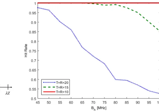
The narrowband assumption A5 leads to a trade-off be-tween azimuth and range resolution, by requiring either small aperture Z or small total bandwidth Btot, respectively. In CDMA, Btot = Bh so that A5 limits the total bandwidth of the waveforms hm(t) [33]. This is illustrated in Fig. 3 which shows the performance of CDMA waveforms using the classical processing detailed below. We use bandlimited Gaussian pulses that are equivalent to CDMA, where each transmitter radiatesP = 1 pulse, and consider range-azimuth recovery in the absence of noise. We assume L = 5 targets whose locations are generated uniformly at random, and adopt a hit-or-miss criterion as our performance metric. A “hit” is defined as a range-azimuth estimate which is identical to the true target position up to one Nyquist bin (grid point) defined
Fig. 3. Hit rate of MIMO radar with classical processing of CDMA waveforms with respect to total bandwidthBtot=Bhand apertureZ=T R/2.
as 1/Btot and2/T R for the range and azimuth, respectively. Each experiment is repeated over 200 realizations. It can be seen that the recovery performance decreases with either increased bandwidth or aperture since in both casesA5 does not hold. In the next section, we show that in FDMA, this assumption can be relaxed under appropriate processing so that the aperture is required to be smaller than the reciprocal of Bh rather thanBtot=T Bh as in (8).
C. Range-Azimuth-Doppler Recovery
Classic collocated MIMO radar processing traditionally includes the following stages:
1) Sampling:at each receiver, the signalxq(t)is sampled at its Nyquist rate Btot.
2) Matched filter: the sampled signal is convolved with a sampled version of hm(t), for 0 ≤ m ≤ T −1. The time resolution attained in this step is 1/Bh. In FDMA, this step leads to a limitation on the range resolution to a single channel bandwidth rather than the total bandwidth.
3) Beamforming: correlations between the observation vectors from the previous step and steering vectors corresponding to each azimuth on the grid defined by the array aperture are computed. The spatial resolution at-tained in this step is2/T R. In FDMA, this stage leads to range-azimuth coupling, as illustrated in Section III-D. 4) Doppler detection: correlations between the resulting
vectors and Doppler vectors, with Doppler frequencies lying on the grid defined by the number of pulses, are computed. The Doppler resolution is1/P τ.
5) Peak detection: a heuristic detection process is per-formed on the resulting range-azimuth-Doppler map. For example, the detection can follow a threshold approach [26] or select the L strongest point of the map, if the number of targets Lis known.
yields a trade-off between azimuth and range resolution. Sec-ond, achieving orthogonality through code design has proven to be a challenging task [2]. To illustrate this, we consider a set of orthogonal bandlimited Gaussian waveforms, generated using a random search for minimizing the cross-correlation between pairs of waveforms. That is, the set of waveforms is constructed so that to minimize the maximal cross-correlation between waveforms, through a non-exhaustive search. Figure 4 shows the maximal cross-correlations between any pair of signals within the set. It can be seen that, when either the bandwidth Bh is reduced or the number of transmit antennas increases, the maximal cross correlation of the CDMA wave-forms increases.
Fig. 4. Maximal cross-correlation of CDMA waveforms using Tp =
0.44µsec with respect to signal bandwidthBhwithT = 20transmitters (top)
and number of transmittersT with bandwidthBh= 100MHz (bottom).
Meanwhile, classic FDMA has been almost neglected owing to its two main drawbacks. First, due to the linear relationship between the carrier frequency and the index of antenna ele-ment, a strong range-azimuth coupling occurs [16], [18], [19], as we illustrate in Section III-D. To resolve this aliasing, the authors in [21] use random carrier frequencies, which creates high sidelobe levels. The second drawback of FDMA is that
the range resolution is limited to a single waveform’s band-width, namelyBh, rather than the overall transmit bandwidth
Btot=T Bh [22], [23].
In the next section, we adopt the FDMA approach, in order to exploit the narrowband property of each individual channel to achieve both high range and azimuth resolution. To resolve the coupling issue, we randomly distribute the antennas, while keeping the carrier frequencies on a grid with spacingBh. In the simulations, we show that random antenna locations yield smaller sidelobes than random carriers. Next, by processing the channels jointly, we achieve a range resolution of1/Btot=
1/T Bh rather than 1/Bh. This way, we exploit the overall received bandwidth that governs the range resolution, while maintaining the narrowband assumption for each channel, which is key to high azimuth resolution. In addition, no code design is required, which may be a challenging task [2], as shown in Fig. 4.
III. FDMA SYSTEM
In this section, we describe our MIMO system based on joint channel processing of FDMA waveforms. Our FDMA processing differs from the classic CDMA approach intro-duced in Section II in several aspects. First, the single channel processing, which is equivalent to matched filtering in step (2), is limited to1/Bh whereas in FDMA we achieve resolution of 1/T Bh. In addition, in FDMA the range depends on the channels while in CDMA, it is decoupled from the channels domain. Therefore, our processing involves range-azimuth beamforming while the classic approach for CDMA uses beamforming on the azimuth domain only as in step (3). The range dependency on the channels in FDMA is exploited to enhance the poor range resolution of the single channel1/Bh to 1/T Bh = 1/Btot, as explained in the remainder of this section. Finally, combining the use of FDMA waveforms with our proposed processing reconciles the narrowband assump-tion with large total bandwidth for range resoluassump-tion, enhancing range-azimuth resolution capabilities.
A. Received Signal Model
Our processing, described in Section IV-B, allows to soften the strict neglect of the delay term in the transition from (12) to (13). We only remove ηmqϑl, that stems from the array geometry, from the envelope h0(t)rather than hm(t). Then, (13) becomes
hm(t−pτ−τl)ej2πfmηmqϑl. (15) Here, the restrictive assumptionA5 is relaxed to 2Zλc ≪ 1
Bh.
The received signal at the qth antenna after demodulation to baseband is in turn given by
xq(t) = neglecting the delay term only in the narrowband envelope
h0(t), (16) results in the extra termej2π(ζq+ξm)ϑlfmλ/c. This corrects the time of arrival differences between channels, so that the narrowband assumptionA5is required only on h0(t) with bandwidth Bh and not on the entire bandwidth Btot. Intuitively, the waveforms are aligned to eliminate the arrival differences resulting from the array geometry with respect to
fm, thus enabling to detect the azimuth with respect to the central carrier fc.
It will be convenient to express xq(t) as a sum of single
Our goal is to estimate the targets range, azimuth and velocity, i.e. to estimate τl,ϑl andflD from xq(t).
B. Frequency Domain Analysis
We begin by deriving an expression for the Fourier coef-ficients of the received signal, and show how the unknown parameters, namely τl, ϑl and flD are embodied in these coefficients. We next turn to range-azimuth beamforming and its underlying resolution capabilities and discuss the range-azimuth coupling. Finally, we present our proposed recovery algorithm, which is based on FDMA waveforms. To introduce our processing, we start with the special case ofP = 1, namely a single pulse is transmitted by each transmit antenna. We show how the range-azimuth map can be recovered from the Fourier coefficients in time and space. Subsequently, we treat the general case where a train of P >1 pulses is transmitted by each antenna, and present a joint range-azimuth-Doppler recovery algorithm from the Fourier coefficients.
The pth frame of the received signal at the qth antenna, namelyxp
q(t), is limited tot∈[pτ,(p+ 1)τ]and thus can be represented by its Fourier series
xp Once the Fourier coefficientscp
q[k]are computed, we sepa-rate them into channels for each transmitter, by exploiting the
fact that they do not overlap in frequency. Applying a matched filter, we have and aligned Fourier coefficients of the channel between the
mth transmitter and qth receiver. Then,
ypm,q[k] =
Let us now pause to discuss the range and azimuth reso-lution capabilities of the described model and processing as well as the coupling issue between the two parameters. Since the Doppler frequency is decoupled from the range-azimuth domain, we assume thatP = 1for the sake of clarity. Then, (22) can be simplified to
ym,q[k] = term and its resolution is related to the virtual array geometry governed byβmq as discussed in [15]. The delay is embodied in the second and third terms, which allows both high range resolution and large unambiguous range. The second term leads to a poor range resolution of 1/Bh corresponding to a single channel, while the resolution induced by the third term, which measures the effect of the delay on the transmit carrier, is dictated by the total bandwidth, namely 1/T Bh. On the other hand, since fm is a multiple of Bh in our configuration, the last term is periodic in τl with a limited period of1/Bh, whereas the second term is periodic inτlwith periodτso that the corresponding unambiguous range iscτ /2. Therefore, by jointly processing both terms we overcome the resolution and ambiguous range limitations and thus achieve a range resolution of 1/T Bh with unambiguous range of τ, as summarized in Table I.
Both the first and third terms, which contain the azimuth and delay respectively, depend on the channels indexed by
TABLE I
RANGERESOLUTION ANDAMBIGUITY
Term Range
Resolution
Unambiguous Range
e−j 2π
τ kτl 1/Bh τ
e−j2πfmτl 1/T Bh 1/Bh
Joint
Processing 1/T Bh τ
single channel processing with range-azimuth beamforming yields joint range-azimuth recovery (Fig. 5(c)). Note that the processing is not divided into these two steps, which are provided for illustration purposes only.
Fig. 5. Illustration of the resolution obtained by processing a single channel and by joint processing of all channels, using range-azimuth beamforming.
D. Range-Azimuth Coupling
As explained above, range-azimuth beamforming over the channels involves the estimation of both parameters from one dimension, the channel dimension. Therefore, it requires a one-to-one correspondence between the phases over the channels to range-azimuth pairs in order to prevent coupling. This ensures that each phase over the channels, expressed by the first and third terms of (23), corresponds to a unique azimuth-range
Fig. 6. Range-azimuth map in noiseless settings for antennas located on the conventional ULA and carrier frequencies selected on a grid, with L= 1
target. The highest peak with the red circle corresponds to the true target. The other peaks results from the range-azimuth coupling.
pair. We next illustrate the range-azimuth coupling which occurs, in particular, in the case where the antennas are located according to the conventional virtual ULA structure shown in Fig. 1, and the carrier frequencies are selected on a grid such that fm= (m−T−21)Bh.
In the single pulse case, whereP = 1, we can rewrite (23) with respect to the channelγ=mR+qas
yγ[k] = L X
l=1
alej2πβγϑle−j2πfγτle−j
2π
τkτl, (24)
whereβγ =γ/2,fγ = (γ modT)Bhandalis equal toαlup to constant phases. Assume that τl andϑl lie on the Nyquist grid such that
τl = τ
T Nsl, ϑl = −1 +
2
T Rrl, (25)
whereslandrl are integers satisfying0≤sl≤T N−1 and
0≤rl≤T R−1, respectively. Then, (24) becomes
yγ[k] = L X
l=1
alej2π
γ
T R(rl−slR)e−jT N2πksl, (26)
for −N
2 ≤ k ≤ N
IV. RANGE-AZIMUTH-DOPPLERRECOVERY
We now describe our recovery approach from the Fourier coefficients of the FDMA received waveforms (16). We first consider the case where P = 1 and derive range-azimuth recovery from the coefficients (23). We next turn to range-azimuth-Doppler recovery from (22).
A. Range-Azimuth Recovery
In practice, as in traditional MIMO, suppose we now limit ourselves to the Nyquist grid with respect to the total bandwidth T Bh so that τl and ϑl lie on the grid defined in
Our goal is to recover X from the measurement matrices Ym,0≤m≤M−1. The time and spatial resolution induced
T R, respectively, as in classic CDMA processing.
Define
A= [A0TA1T · · · A(T−1)T]T, (28)
and
B= [B0TB1T · · · B(T−1)T]T. (29)
To better grasp the structure of A and B, suppose that the
carriersfmlie on the gridfm= (m−T−21)Bh. In this case, the (k, n)th element ofAm ise−jT N2π(k+mN−T N2 )n andAis
theT N×T NFourier matrix up to row permutation. Similarly, assuming that the antenna elements lie on the virtual array illustrated in Fig. 1, we have βmq = 12(q +mR), where we used A5 to simplify the expression. Then, the (q, p)th element ofBmisejT R2π(q+mR)(p−
T R
2 )andBis theT R×T R
Fourier matrix up to column permutation. The matricesAand B are sometimes referred to as dictionaries, whose columns
correspond to the range and azimuth grid points, respectively. However, this configuration leads to range-azimuth coupling as discussed in Section III-D. In Section V, we use a random array to avoid range-azimuth coupling.
One approach to solving (27) is based on CS [50], [39] techniques that exploits the sparsity of the target scene. One of CS recovery advantages is that it allows to reduce the number of required samples, pulses and channels while preserving the underlying resolution [51]. In particular, we adopt an itera-tive reconstruction approach that is beneficial when dealing with high dynamic range with both weak and strong targets, especially since the sidelobes are slightly raised due to the random array configuration. Our recovery algorithm is based on orthogonal matching pursuit (OMP) [50], [39]. Similar subtraction techniques are used in many iterative algorithms such as the CLEAN process [52].
To recover the sparse matrix X from the set of equations
(27), for all 0 ≤m ≤M −1, where the targets’ range and azimuth lie on the Nyquist grid, we consider the following optimization problem
min||X||0 s.t. AmX(Bm)T =Ym, 0≤m≤T−1.
(30) It has been shown in [51] that the minimal number of channels required for perfect recovery of X in (30) with L targets in
noiseless settings is T R ≥ 2L with a minimal number of
T N ≥2Lsamples per receiver. To solve (30), we extend the matrix OMP from [53] to simultaneously solve a system of CS matrix equations, as shown in Algorithm 1. In the algo-rithm description, vec(Y),
recovered, the delays and azimuths are estimated as
ˆ
Other CS recovery algorithms, such as FISTA [54], [55], can
Algorithm 1 Simultaneous sparse 2D recovery based OMP Input: Observation matrices Ym, measurement matrices
Am,Bm, for all0≤m≤T −1
Output: Index setΛcontaining the locations of the non zero indices of X, estimate for sparse matrixXˆ
1: Initialization: residual Rm0 = Ym, index set Λ0 = ∅, t= 1
2: Project residual onto measurement matrices:
Ψ=AHR ¯B
whereAandBare defined in (28) and (29), respectively,
andR=diag [R0t−1 · · ·RTt−−11]
is block diagonal
3: Find the two indices λt= [λt(1) λt(2)]such that
[λt(1) λt(2)] = arg maxi,j|Ψi,j|
4: Augment index setΛt= ΛtS{λt}
5: Find the new signal estimate
ˆ
7: Ift < L, incrementt and return to step 2, otherwise stop
8: Estimated support setΛ = Λˆ L
9: Estimated matrixXˆ:(ΛL(l,1),ΛL(l,2))-th component of ˆ
X is given by αˆl for l = 1,· · · , L while rest of the
elements are zero
The projection performed in step 2 of the algorithm com-bines single channel processing with range-azimuth beam-forming. The former coherently processes the second term of (23), which appears in the matrix A, while range-azimuth
beamforming over the channels coherently processes the first and third terms of (23), which are contained in AandB,
re-spectively. The FDMA narrowband assumption reconciliation is due to the additional third term of (15), contained in B,
thus enhancing range-azimuth resolution capabilities.
The improved performance of the iterative approach over non-iterative target recovery with high dynamic range is illus-trated in simulations in Section V. There, we also compare our FDMA approach with classic CDMA, when using a non-iterative recovery method in the former. In particular, we only use one iteration of Algorithm 1, which is equivalent to the classic approach. This demonstrates that our FDMA method outperforms CDMA due to the high range-azimuth resolu-tion capabilities stemming from the reconciliaresolu-tion between the individual narrowband assumption and the large overall bandwidth.
B. Range-Azimuth-Doppler Recovery
Besides τl and ϑl lying on the grid defined in (25), we assume that the Doppler frequency fD
l is limited to the Nyquist grid as well, defined by the CPI as:
flD=− be the N R×P matrix withqth column given by the vertical concatenation of yp
are defined as in Section IV-A and F denotes the P ×P
Fourier matrix up to column permutation. The matrix XD is
aT2N R×P sparse matrix that contains the valuesα l at the
L indices(rlT N+sl, ul).
Our goal is now to recover XD from the measurement
matricesZm,0≤m≤T−1. The time, spatial and frequency resolution stipulated byXD are τ
T N =
P τ respectively, as in classic CDMA processing. To jointly recover the range, azimuth and Doppler frequency of the targets, we apply the concept of Doppler focusing from [56] to our setting. Once the Fourier coefficients (22) are processed, we perform Doppler focusing for a specific frequencyν, that is
Φνm,q[k] =
2 −1. Following the same argument as in [56], it holds that
Therefore, for each focused frequencyν, (35) reduces to a 2-dimensional problem. We note that Doppler focusing increases the SNR by a factor a P, as can be seen in (36).
Algorithm 2 solves (34) for 0 ≤ m ≤ T − 1 using Doppler focusing. Note that step 1 can be performed using the fast Fourier transform (FFT). In the algorithm descrip-tion, vec(Z) is defined as in the previous section, et(l) =
imuths are given by (31) and (32), respectively, and the Doppler frequencies are estimated as
ˆ
Similarly to the one-pulse case, the minimal number of chan-nels required for perfect recovery of XD with L targets in
noiseless settings is T R ≥ 2L with a minimal number of
T N ≥ 2L samples per receiver and P ≥ 2L pulses per transmitter [51].
V. SIMULATIONS
In this section, we present numerical experiments illustrat-ing our FDMA approach and compare our method with classic MIMO processing using CDMA.
A. Preliminaries
Throughout the experiments, the standard MIMO system is based on a virtual array, as depicted in Fig. 1 generated by T = 20 transmit antennas and R = 20 receive antennas, yielding an aperture λZ = 6m. We consider a random array configuration where the transmitters and receivers’ locations are selected uniformly at random over the apertureZ. We use FDMA waveforms hm(t) such that fm = (im− T−21)Bh, whereim are integers chosen uniformly at random in [0, T), for 0 ≤ m ≤ T − 1, and all frequency bands within
[−T2Bh,T2Bh] are used for transmission. We consider the following parameters: PRI τ = 100µsec, bandwidth Bh =
5M Hz and carrier frequency fc = 10GHz. We simulate targets from the Swerling-0 model with identical amplitudes and random phases. The received signals are corrupted by uncorrelated additive Gaussian noise (AWGN) with power spectral densityN0. The SNR is defined as
SNR=
whereTp is the pulse time.
Algorithm 2 Simultaneous sparse 3D recovery based OMP with focusing
Input: Observation matrices Zm, measurement matrices Am,Bm, for all0≤m≤T−1
Output: Index setΛcontaining the locations of the non zero indices ofXD, estimate for sparse matrixXˆD
1: Perform Doppler focusing for 0 ≤i≤N −1,0 ≤j ≤
R−1and0≤ν ≤P−1:
Φ(m,ν)
i,j = (ZmF¯)i+jN,ν.
2: Initialization: residual R(m,ν)0 =Φ(m,ν), index setΛ0=
∅,t= 1
3: Project residual onto measurement matrices for0 ≤ν ≤
P−1:
Ψν =AHRνB¯,
whereAandBare defined in (28) and (29), respectively,
andRν =diag[R(0,ν) t−1 · · · R
(T−1,ν) t−1 ]
is block diagonal
4: Find the three indicesλt= [λt(1)λt(2)λt(3)]such that
[λt(1) λt(2) λt(3)] = arg maxi,j,ν Ψνi,j
5: Augment index setΛt= ΛtS{λt}
6: Find the new signal estimate
ˆ
α= [ˆα1. . . αˆt]T = (EtTEt)−1ETtvec(Z)
7: Compute new residual
R(m,ν)
t =R (m,ν)
0 −
t X
l=1
αlamΛt(l,1)
bm
Λt(l,2)
T
fΛ
t(l,3)
Tf ν
8: Ift < L, increment tand return to step 3, otherwise stop
9: Estimated support setΛ = Λˆ L
10: Estimated matrix XˆD:
(ΛL(l,2)T N+ ΛL(l,1),ΛL(l,3))-th component of
ˆ
XD is given by αˆl for l = 1,· · ·, L while rest of the
elements are zero
defined as 1/T Bh and 2/T R for the range and azimuth, respectively. In pulse-Doppler settings, a “hit” is proclaimed if the recovered Doppler is identical to the true frequency up to one Nyquist bin of size1/P τ, in addition to the two previous conditions.
B. Numerical Results
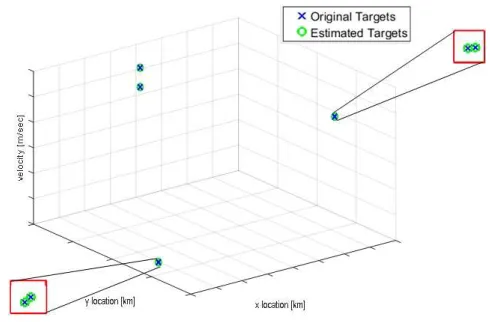
We first consider a sparse target scene with L = 6targets including a couple of targets with close ranges, a couple with close azimuths and another couple with close velocities. We use P = 10 pulses and the SNR is set to −10dB. As can be seen in Fig. 7, all targets are perfectly recovered, demonstrating high resolution in all dimensions. Here, the range and azimuth are converted to 2-dimensional x and y
locations.
We next turn to the range-azimuth coupling issue and dis-cuss the impact of the choice of antennas’ locations and trans-missions’ carrier frequencies. As discussed in Section III-D, the conventional ULA array structure shown in Fig. 1 with carrier frequency selected on a grid, leads to ambiguity in
Fig. 7. Range-azimuth-Doppler recovery forL= 6targets and SNR=−10dB.
Fig. 8. Range-azimuth map in noiseless settings for random carrier frequen-cies along range axis (a) and azimuth axis (b), and for random antennas’ locations along range axis (c) and azimuth axis (d), forL= 1target. The
red dotted line indicates the peak sidelobe level for this target.
the range-azimuth domain. In order to overcome the ambi-guity issue, we adopt a random array configuration [38]. We found heuristically that a configuration with random antennas’ locations with carriers on a grid provides better results than random carriers with a ULA structure. Figure 8 shows a typical result of sidelobes for both configurations. The peak sidelobe level for the configuration with random antennas’ locations is consistently lower.
Fig. 9. Hit rate of FDMA and classic CDMA versus bandwidth.
Fig. 10. Range-azimuth recovery forL= 4targets using classic CDMA (a)
and FDMA (b) .
azimuth angle θl are detected by both techniques, whereas targets on the end-fire direction (θl = ±90◦, corresponds to the broadside direction) are missed by the CDMA approach. This happens because the delay differences between channels are too large, which violates the narrowband assumptionA5. In order to demonstrate that the performance gain of our FDMA approach over the classic CDMA is due to the re-laxed narrowband assumption rather than our specific iterative processing, we consider a non-iterative recovery approach. Figure 11 shows our FDMA method with non-iterative recov-ery, corresponding to one iteration of Algorithm 1. This con-stitutes evidence that our approach outperforms conventional CDMA processing from the relaxed narrowband assumption.
The iterative approach does boost performance of multiple targets recovery with high RCS dynamic range, allowing detection of weak targets masked by the strong ones. In doing so, we further decrease the effect of the sidelobe level and thus improve detection performance. To compare both iterative and non iterative recovery, we consider L= 2 targets whose locations are generated uniformly at random with varying RCS ratios defined as10 log10
α
lmax
αlmin
. In Fig. 12, we can see that the non-iterative approach attains50%hit rate for an RCS ratio of 8 dB, which means that the weak target is totally masked by
Fig. 11. Hit rate of non-iterative FDMA and classic CDMA versus bandwidth.
Fig. 12. Hit rate of iterative FDMA and non-iterative FDMA versus RCS ratio.
the strong one. The iterative approach detects the weak target up to an RCS ratio of 20 dB.
Each iteration of our proposed FDMA approach takes 3.9 sec for 40 million range-azimuth-Doppler grid points using an Intel Core i7 PC without GPU components. We have im-plemented a hardware prototype realizing the FDMA MIMO processing presented here. The prototype, shown in Fig. 13, proves the hardware feasibility of our FDMA MIMO radar. Further details can be found in [57], [58].
VI. CONCLUSION
Fig. 13. FDMA MIMO prototype and user interface [58].
In order to overcome one of the main FDMA’s drawbacks, that limits the range resolution to the individual bandwidth, we proposed a joint processing algorithm of the channels achieving range resolution with respect to the overall band-width. A large virtual array aperture, that yields high azimuth resolution, is enabled by the relaxed narrowband assumption and appropriate digital processing. Our system and subsequent processing copes with range-azimuth coupling, which occurs when using FDMA, by using a random array configuration. The digital processing is a feasible iterative CS based approach for simultaneous sparse recovery. Simulations illustrated the increased resolution obtained by our approach in comparison with classic CDMA, leading to better detection performance.
REFERENCES
[1] E. Fishler, A. Haimovich, R. Blum, D. Chizhik, L. Cimini, and R. Valen-zuela, “MIMO radar: an idea whose time has come,” inIEEE Radar Conf., 2004, pp. 71–78.
[2] J. Li and P. Stoica, MIMO radar signal processing. Wiley Online Library, 2009.
[3] M. Lesturgie, “Some relevant applications of MIMO to radar,” inIEEE Int. Radar Symposium. IEEE, 2011, pp. 714–721.
[4] A. Martinez-Vazquez and J. Fortuny-Guasch, “UWB MIMO radar arrays for small area surveillance applications,” inIET European Conf. Antennas and Propagation. IET, 2007, pp. 1–6.
[5] S. Lutz, K. Baur, and T. Walter, “77 GHz lens-based multistatic MIMO radar with colocated antennas for automotive applications,” inIEEE Int. Microwave Symposium Digest. IEEE, 2012, pp. 1–3.
[6] K. Schuler, M. Younis, R. Lenz, and W. Wiesbeck, “Array design for automotive digital beamforming radar system,” inIEEE Int. Radar Conf. IEEE, 2005, pp. 435–440.
[7] J.-H. Kim, A. Ossowska, and W. Wiesbeck, “Investigation of MIMO SAR for interferometry,” inIEEE European Radar Conf. IEEE, 2007, pp. 51–54.
[8] S. Anderson and W. Anderson, “A MIMO technique for enhanced clutter selectivity in a multiple scattering environment: Application to hf surface wave radar,” inInt. Conf. Electromagnetics in Advanced Applications, 2010.
[9] X. P. Masbernat, M. G. Amin, F. Ahmad, and C. Ioana, “An MIMO-MTI approach for through-the-wall radar imaging applications,” inIEEE Int. Waveform Diversity and Design Conf. IEEE, 2010, pp. 188–192. [10] E. Pancera, T. Zwick, and W. Wiesbeck, “Ultra wideband radar imaging:
An approach to monitor the water accumulation in the human body,” in IEEE Int. Conf. Wireless Inf. Technology and Syst. IEEE, 2010, pp. 1–4.
[11] J. Li and P. Stoica, “MIMO radar with collocated antennas,”IEEE Signal Process. Mag., vol. 24, no. 5, pp. 106–114, 2007.
[12] A. M. Haimovich, R. S. Blum, and L. J. Cimini, “MIMO radar with widely separated antennas,”IEEE Signal Process. Mag., vol. 25, no. 1, pp. 116–129, 2008.
[13] D. Bliss and K. Forsythe, “Multiple-input multiple-output (MIMO) radar and imaging: degrees of freedom and resolution,” in IEEE Asilomar Conf. Signals, Syst. and Computers, vol. 1. IEEE, 2003, pp. 54–59.
[14] D. J. Rabideau and P. Parker, “Ubiquitous MIMO multifunction digital array radar,” in IEEE Asilomar Conf. Signals, Syst. and Computers, vol. 1. IEEE, 2003, pp. 1057–1064.
[15] J. Li and P. Stoica, “MIMO radar diversity means superiority,” in Adaptive Sensor Array Process. Workshop. Lincoln Lab, 2009. [16] M. Cattenoz, “MIMO radar processing methods for anticipating and
preventing real world imperfections,” Ph.D. dissertation, Universit´e Paris Sud-Paris XI, 2015.
[17] F. Gini, Waveform design and diversity for advanced radar systems. The Institution of Engineering and Technology, 2012.
[18] O. Rabaste, L. Savy, M. Cattenoz, and J.-P. Guyvarch, “Signal wave-forms and range/angle coupling in coherent colocated MIMO radar,” in IEEE Int. Conf. Radar, 2013, pp. 157–162.
[19] H. Sun, F. Brigui, and M. Lesturgie, “Analysis and comparison of MIMO radar waveforms,” inIEEE Int. Radar Conf. IEEE, 2014.
[20] J. H. Ender and J. Klare, “System architectures and algorithms for radar imaging by MIMO-SAR,” inIEEE Int. Radar Conf. IEEE, 2009. [21] J. Dorey and G. Garnier, “RIAS, synthetic impulse and antenna radar,”
ONDE ELECTRIQUE, vol. 69, pp. 36–44, 1989.
[22] J. P. Stralka, R. M. Thompson, J. Scanlan, and A. Jones, “MISO radar beamforming demonstration,” in IEEE RadarCon. IEEE, 2011, pp. 889–894.
[23] P. Vaidyanathan and P. Pal, “MIMO radar, SIMO radar, and IFIR radar: a comparison,”Asilomar Conf. Signals, Syst. and Computers, pp. 160– 167, 2009.
[24] B. Donnet and I. Longstaff, “MIMO radar, techniques and opportuni-ties,” inIEEE European Radar Conf. IEEE, 2006, pp. 112–115. [25] ——, “Combining MIMO radar with OFDM communications,” inIEEE
European Radar Conf. IEEE, 2006, pp. 37–40.
[26] M. A. Richards, Fundamentals of radar signal processing. Tata McGraw-Hill Education, 2014.
[27] N. Levanon and E. Mozeson,Radar signals. John Wiley & Sons, 2004. [28] D. R. Wehner,High resolution radar. Norwood, MA, Artech House,
Inc., 1987.
[29] R. T. Lord, “Aspects of stepped-frequency processing for low-frequency sar systems,” Ph.D. dissertation, University of Cape Town, 2000. [30] R. Barker, “Group synchronizing of binary digital systems,” Comm.
Theory, pp. 273–287, 1953.
[31] D. Tse and P. Viswanath, Fundamentals of wireless communication. Cambridge university press, 2005.
[32] R. Gold, “Optimal binary sequences for spread spectrum multiplexing (corresp.),”IEEE Trans. Inf. Theory, vol. 13, no. 4, pp. 619–621, 1967. [33] P. Vaidyanathan, P. Pal, and C.-Y. Chen, “MIMO radar with broadband waveforms: Smearing filter banks and 2D virtual arrays,”Asilomar Conf. Signals, Syst. and Computers, pp. 188–192, 2008.
[34] D. B. Ward, R. A. Kennedy, and R. C. Williamson, “Theory and design of broadband sensor arrays with frequency invariant far-field beam patterns,” The Journal of the Acoustical Society of America, vol. 97, no. 2, pp. 1023–1034, 1995.
[35] T. Chou, “Frequency-independent beamformer with low response error,” in Acoustics, Speech, and Signal Processing, 1995. ICASSP-95., 1995 International Conference on, vol. 5. IEEE, 1995, pp. 2995–2998. [36] W. Liu and S. Weiss, “New class of broadband arrays with frequency
invariant beam patterns,” inAcoustics, Speech, and Signal Processing, 2004. Proceedings.(ICASSP’04). IEEE International Conference on, vol. 2. IEEE, 2004, pp. ii–185.
[37] Y. Lo, “A mathematical theory of antenna arrays with randomly spaced elements,” IEEE Transactions on Antennas and Propagation, vol. 12, no. 3, pp. 257–268, 1964.
[38] M. Rossi, A. M. Haimovich, and Y. C. Eldar, “Spatial compressive sensing for MIMO radar,”IEEE Trans. Signal Process., vol. 62, no. 2, pp. 419–430, 2014.
[39] Y. C. Eldar,Sampling Theory: Beyond Bandlimited Systems. Cambridge University Press, 2015.
[40] J. Xu, G. Liao, S. Zhu, L. Huang, and H. C. So, “Joint range and angle estimation using MIMO radar with frequency diverse array,”IEEE Trans. Signal Process., vol. 63, no. 13, pp. 3396–3410, 2015.
[41] W.-Q. Wang, “Space-time coding MIMO-OFDM SAR for high-resolution imaging,” IEEE Trans. Geoscience and Remote Sensing, vol. 49, no. 8, pp. 3094–3104, 2011.
[42] S. Sen and A. Nehorai, “Adaptive OFDM radar for target detection in multipath scenarios,”IEEE Trans. Signal Process., vol. 59, no. 1, pp. 78–90, 2011.
[43] M. Skolnik,Radar handbook. McGraw Hill, 1970.
[45] D. L. Mensa, “Wideband radar cross section diagnostic measurements,” IEEE Trans. Instrumentation and Measurement, vol. 33, no. 3, pp. 206– 214, 1984.
[46] C.-Y. Chen, “Signal processing algorithms for MIMO radar,” Ph.D. dissertation, California Institute of Technology, 2009.
[47] P. Z. Peebles,Radar principles. John Wiley & Sons, 2007.
[48] O. Rabaste, L. Savy, M. Cattenoz, and J.-P. Guyvarch, “Signal wave-forms and range/angle coupling in coherent colocated MIMO radar,” IEEE Int. Conf. Radar, pp. 157–162, Sept. 2013.
[49] E. Fishler, A. Haimovich, R. S. Blum, and L. J. Cimini, “Spatial diversity in radars-models and detection performance,” IEEE Trans. Signal Process., vol. 54, pp. 823–838, Mar. 2006.
[50] Y. C. Eldar and G. Kutyniok,Compressed Sensing: Theory and Appli-cations. Cambridge University Press, 2012.
[51] D. Cohen, D. Cohen, Y. C. Eldar, and A. M. Haimovich, “SUMMeR: sub-Nyquist MIMO radar,” 2016.
[52] J. Tsao and B. D. Steinberg, “Reduction of sidelobe and speckle artifacts in microwave imaging: the CLEAN technique,”IEEE Trans. Antennas and Propagation, vol. 36, no. 4, pp. 543–556, 1988.
[53] T. Wimalajeewa, Y. C. Eldar, and K. P., “Recovery of sparse matrices via matrix sketching,” CoRR, vol. abs/1311.2448, 2013. [Online]. Available: http://arxiv.org/abs/1311.2448
[54] A. Beck and M. Teboulle, “A fast iterative shrinkage-thresholding algorithm for linear inverse problems,”SIAM J. Imaging Sciences, vol. 2, pp. 183–202, 2009.
[55] D. P. Palomar and Y. C. Eldar,Convex Optimization in Signal Processing and Communications. Cambridge University Press, 2010.
[56] O. Bar-Ilan and Y. C. Eldar, “Sub-Nyquist radar via Doppler focusing,” IEEE Trans. Signal Process., vol. 62, no. 7, pp. 1796–1811, 2014. [57] K. V. Mishra, E. Shoshan, M. Namer, M. Meltsin, D. Cohen, R.


![Fig. 13. FDMA MIMO prototype and user interface [58].](https://thumb-ap.123doks.com/thumbv2/123dok/2119836.1609768/12.612.50.315.57.165/fig-fdma-mimo-prototype-and-user-interface.webp)
