Hybrid Model GSTAR-SUR-NN For Precipitation Data
Agus Dwi Sulistyono, Waego Hadi Nugroho, Rahma Fitriani, Atiek Iriany
Department of Statistics, Faculty of Mathematics and Natural Sciences Brawijaya University, Malang
Email: [email protected], [email protected]
ABSTRACT
Spatio-temporal model that have been developed such as Space-Time Autoregressive (STAR) model, Generalized Space-Time Autoregressive (GSTAR), GSTAR-OLS and GSTAR-SUR. Besides spatio-temporal phenomena, in daily life, we often find nonlinear phenomena, uncommon patterns and unidentified characteristics of the data. One of current developed nonlinear model is a neural network. This study is conducted to form a hybrid model GSTAR-SUR-NN to develop spatio-temporal model that has better prediction. This research is conducted on ten-daily rainfall data at 2005 - 2015 for Blimbing, Singosari, Karangploso, Dau, and Wagir region. Based on the results of this research, indicated that the accuracy of GSTAR ((1), 1,2,3,12,36)-SUR model used cross-covariance weight has relatively similar to GSTAR ((1), 1,2,3 , 12.36)-SUR-NN (25-14-5) for Blimbing and Singosari region with 5% error level. While Karangploso, Dau, and Wagir, GSTAR ((1), 1,2,3,12,36)-SUR-NN (25-14-5) model has better accuracy in predicting the precipitation at three locations with the value of R2prediction for each location is 0.992, 0.580, and 0.474.
Keywords: spatio temporal, precipitation, hybrid model, neural network
INTRODUCTION
One of the spatio-temporal model that has been developed is Space-Time Autoregressive (STAR) which introduced by Pfeifer and Deutsch[1]. STAR model did not fit for the data which had heterogeneous characteristics of locations. It was the STAR model's weaknesses and it can be addressed by the Generalized Space-Time Autoregressive (GSTAR) model and GSTAR-OLS that developed by Ruchjana[2], [3]. The latest development of spatio-temporal models is GSTAR-SUR developed by Iriany [4] to address for non-stationary and seasonal pattern data.
The use of locations weights on the formation of spatio temporal models also contribute to the accuracy of the model. The location weights that often used are uniform weight, inverse distance, and normalized cross correlation weight [5], [6]. The location weight consider the neighborhood between locations. For data that has a high variability, it is necessary to consider the location weight with variability aspects of observational data, cross covariance weights. The use of cross covariance weights have been studied and applied by Apanasovich and Genton [7] to predict pollution in California and Efromovich and Smirnova [8] to process the fMRI imaging with wavelate approach.
and difficult to do on the data with nonlinear pattern. Some nonlinear time series models have been developed and applied by Tong [9], Priestley [10], Lee et al. [11], as well as Granger and Terasvirta [12]. Nonlinear time series model that most developed and applied is Artificial Neural Network. Therefore, this study was conducted to form a hybrid model GSTAR-SUR-NN to develop spatio-temporal models that have better forecasts.
THEORITICAL REVIEW
Location Weight
The problems that arise in the modeling of space-time is the use of location weight. There are several methods to determine the weight location in space-time model of the application [6], such as :
a. Uniform Weight
Uniform weights can be calculated using the formula 𝑤𝑖𝑗= 1
𝑛𝑖 with niis the number of
neighborhood locations with ith locations. Weight of the location is only used for homogeneous
characteristics or have the same distance between locations b. Inverse Distance Weight
Inverse distance weight is calculated based on the actual distance between locations. The closer the distance between locations, the greater weight is. Thus, a location adjacent have greater weight.
c. Normalized Cross-Correlation Weight
This weight is the result of the normalization of cross-correlation between the location of the corresponding time lag [5]. The normalization of cross-correlation weight was first introduced by Suhartono and Atok [6] and more applied research by [5].
d. Normalized Cross-Covariance Weight
The use of cross covariance weight had been studied and applied by Apanasovich and Genton [7] to predict pollution in California, as well as Efromovich and Smirnova [8]to process the fMRI imaging with wavelate approach.
GSTAR Model
Ruchjana [3] suggested that GSTAR was a generalization and extension of Space Time Autoregresssive models (STAR) by Pfeifer [1]. The main difference are on spatial dependent and weight matrix. GSTAR more realistic because it is in fact more prevalent models with different parameters for different locations [13]. GSTAR with p order and 𝜆1, 𝜆2, …𝜆𝑝 spatial order, GSTAR
that count the relationship between the equation error. The error value is obtained from the estimated ordinary least squares (OLS) that will be used in the calculation to estimate the regression coefficients in the SUR system equation. SUR models with M equation expressed by:
𝒚𝒊 = 𝑿𝒊𝜷𝒊+ 𝜺𝒊, 𝑖 = 1, … , 𝑁 (8) where 𝒚𝒊 is vector with size R×1, 𝑋𝑖’s size is R×𝑘𝑖 dan 𝛽𝑖 vector with size 𝑘𝑖× 1.
According to Greene [15], equation (8) is SUR model with the assumption 𝐸[𝜀|𝑿𝟏,𝑿𝟐,… , 𝑿𝑵] = 0 and 𝐸[𝜀𝜀′|𝑿𝟏,𝑿𝟐,… , 𝑿𝑵] = 𝛀 with 𝛀 is variance-covariance matrices.
GLS method use the error variance :
Cov(𝜀) = 𝐸(𝜀𝜀′) = σ2𝚺 = 𝛀. Matrix 𝛀 describe the error correlation with :
𝛀 = E(𝜀𝜀′) = [
The parameter model estimation is obtained by estimating parameter 𝜷 in equation (8).
𝜺∗′𝜺∗ = 𝜺′𝛀−𝟏𝛆
Hybrid model by integrating the neural network with conventional forecasting model was proved capable of producing more accurate forecasts. Some hybrid models using neural network are Feed Forward Neural Network for time series data [16], Auto Regressive Integrated Moving Average With Exogenous Factor-Neural Network (ARIMAX-NN) for data Inflation in Indonesia [17], and Neural Network - Multiscale Autoregressive (NN-MAR) for forecasting the number of tourists [18].
RESULTS AND DISCUSSION
Based on the result of descriptive statistics analysis, we can describe the descriptive statistics of precipitation data for each location :
Table 1. Description of Precipitation Data in Five Location
Location N
Mean (mm)
Standard Deviation (mm)
Minimum (mm)
Maximum (mm)
Blimbing 360 5.682 6.909 0 33.5
Singosari 360 3.93 5.575 0 41.75
Karangploso 360 4.302 5.71 0 25.36
Dau 360 4.564 5.825 0 36.38
Wagir 360 7.08 8.187 0 43.63
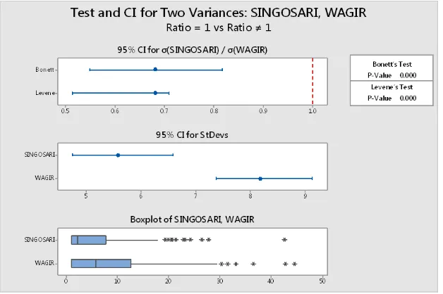
Table 1 shows that precipitation of each location has a high variability. It can be seen that the standard deviation of precipitation of all location greater than the average. High variability indicates that there is fluctuation to the extreme point of precipitation, especially during the rainy season. Here is the result of homogeneity test of variance the precipitation data:
Figure 1. The Result of Homogeneity Test of Variance
Figure 2 describe the results of homogeneity test of variance precipitation data using Bartlett and Levene test that was obtained p-value of 0.000 (p < 0.05), indicating that the precipitation data at Blimbing, Karangploso, Singosari, Wagir, and Dau region have different variance. Model identification is done by comparing the value of AIC at some time lag. Here the value of AIC with VARMAX procedure in SAS:
Table 2. The Value of AIC with VARMAX Procedure
Time Lag AIC Value
1 14.67906
2 14.52868
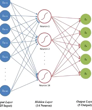
Based on table 2 above, indicated that at the time lag of 1-3, the lowest AIC is in 3rd time lag. Thus, the order GSTAR model is GSTAR ((1), 1,2,3)-SUR. Based on ACF of precipitation data at each location there is seasonal pattern in the time lag of 12 and 36. Therefore, the appropriate model is GSTAR ((1) (1,2,3,12 , 36)) - SUR. The architecture of GSTAR-SUR-NN model is as follows:
Figure 2. The architecture of GSTAR((1),1,2,3,12,36)-SUR-NN (25-14-5) Model
The neural network architecture consist of 25 input variables, 14 hidden layers, dan 5 output layers. Therefore, hybrid model ofGSTAR-SUR-NN is GSTAR((1),1,2,3,12,36)-SUR-NN (25-14-5). Follow is the result of validation test of GSTAR ((1)(1,2,3,12,36))-SUR model and GSTAR((1),1,2,3,12,36)-SUR-NN (25-14-5) model :
Table 3. The Result of GSTAR-SUR and GSTAR-SUR-NN Model Validation Test
Model t-statistics p-value
GSTAR((1),1,2,3,12,36)-SUR 2.619 0.010 GSTAR((1),1,2,3,12,36)-SUR-NN (25-14-5) 0.332 0.741
Based on the results of validation test of GSTAR ((1), 1,2,3,12,36)-SUR using cross
covariance weight in Table 3, showed that, at α = 5%, GSTAR ((1),1,2,3,12,36)-SUR model has p-value less than 0.05 which implies that there is a significant difference between average of actual precipitation data with average of predicted results. Or in other words, GSTAR ((1), 1,2,3,12,36)-SUR using cross-covariance weights still have low accuracy. While, GSTAR ((1), 1,2,3,12,36) -1,2,3,12,36) -SUR-NN (25-14-5) was obtained p-value of 0.741. P-value is more than 0.05 implies that there is no significant difference between the average of actual precipitation with the average precipitation predicted results. Or in other words, GSTAR ((1),1,2,3,12,36)-SUR-NN (25-14-5) model have high accuracy. From this comparison, it has been proven that GSTAR ((1), 1,2,3,12,36)-SUR-NN (25-14-5) model has better accuracy rate in predicting the precipitation data.
Table 4. The Comparison GSTAR-SUR and GSTAR-SUR-NN Model Performance
Location
GSTAR-SUR Model GSTAR-SUR-NN Model
Data Testing
RMSE R2prediction
Data Testing
RMSE R2prediction Blimbing
10.132 0.539 10.672 0.640
Karangploso 0.623 0.992
Dau 0.527 0.580
Wagir 0.365 0.474
Table 4 explains the performance comparison between GSTAR ((1),1,2,3,12,36)-SUR with the hybrid model GSTAR ((1), 1,2,3,12,36)-SUR-NN (25-14 -5). From these comparison, indicated that GSTAR-SUR model has RMSE value lower than the hybrid model GSTAR-SUR-NN. Judging from the value of RMSE, GSTAR-SUR model have better performance because it produces lower RMSE value. But, if it judge from the R2prediction value, indicated that the R2prediction value on
the hybrid model GSTAR-SUR-NN is higher than GSTAR-SUR model. In fact, the R2prediction value
of Karangploso region reached 0.992. Based on this comparison, it is proved that the hybrid model GSTAR ((1),1,2,3,12,36)-SUR-NN (25-14-5) has better accuracy rate in predicting precipitation in Malang especially Blimbing, Singosari, Karangploso, Dau, and Wagir region.
CONCLUSION
Based on the results of this study concluded that the hybrid model GSTAR ((1), 1,2,3,12,36)-SUR-NN (25-14-5) produces precipitation forecast better than GSTAR ((1),1,2,3,12,36)-SUR model.
REFERENCE
[1] P. E. Pfeifer and S. J. Deutsch, “Identification and Interpretation of First Order Space-Time ARMA Models,” Technometrics, vol. 22, no. 3, pp. 397–408, 1980.
[2] B. N. Ruchjana, “Study on the Weight Matrix in the Space-Time Autoregressive Model,” in Proceeding
of the 10th International Symposium on Applied Stochastic Models and Data Analysis (ASMDA), France,
2001, vol. 2, pp. 789–794.
[3] B. N. Ruchjana, “A Generalized Space Time Autoregressive Model and its Application to Oil Production Data,” Institut Teknologi Bandung, Bandung, 2002.
[4] A. Iriany, Suhariningsih, B. N. Ruchjana, and Setiawan, “Prediction of Precipitation Data at Batu Town Using the GSTAR (1,p)-SUR Model,” J. Basic Appl. Sci. Res., vol. 3, no. 6, pp. 860–865, 2013.
[5] S. Suhartono and S. Subanar, “The Optimal Determination Of Space Weight in Gstar Model by Using Cross-Correlation Inference,” Quant. METHODS, vol. 2, no. 2, pp. 45–53, Dec. 2006.
[6] Suhartono and R. M. Atok, “Pemilihan Bobot Lokasi yang Optimal pada Model GSTAR,” in Prosiding
Konferensi Nasional Matematika XIII, Semarang, 2006.
[7] T. V. Apanasovich and M. G. Genton, “Cross-covariance functions for multivariate random fields based on latent dimensions,” Biometrika, vol. 97, no. 1, pp. 15–30, Mar. 2010.
[8] E. Smirnova, “Statistical Analysis of Large Cross-Covariance and Cross-Correlation Matrices Produced by fMRI Images,” J. Biom. Biostat., vol. 5, no. 2, 2013.
[9] H. Tong, Non-Linear Time Series: A Dynamical System Approach. Oxford University Press, 1993. [10] M. B. Priestley, Non-Linear and Non-Stationary Time Series Analysis, 2nd edition, 2nd ed. London:
Academic Press, 1991.
[11] T.-H. Lee, H. White, and C. W. J. Granger, “Testing for neglected nonlinearity in time series models: A comparison of neural network methods and alternative tests,” J. Econom., vol. 56, no. 3, pp. 269–290, Apr. 1993.
[12] C. W. . Granger and T. Terasvirta, Modeling Nonlinear Economic Relationships. United Kingdom: Oxford University Press.
[13] W. Dhoriva Urwatul and S. Suhartono, “PERAMALAN DERET WAKTU MULTIVARIAT SEASONAL PADA DATA PARIWISATA DENGAN MODEL VAR-GSTAR,” in Seminar Nasional Matematika dan Pendidikan
Matematika 2009, 2009.
[14] S. A. Borovkova, H. P. Lopuha, and B. N. Ruchjana, “Generalized S-TAR with Random Weights,” in the
17th International Workshop on Statistical Modeling, Chania-Greece.
[15] W. H. Greene, Econometric analysis, 7th ed. Boston: Prentice Hall, 2012.
[17] H. Suryono, “Auto Regressive Integrated Moving Average With Exogeneous Factor-Neural Network (ARIMAX-NN) pada Data Inflasi di Indonesia,” Institut Teknologi Sepuluh November, Surabaya, 2009. [18] B. Sutijo, S. Suhartono, and A. J Endharta, “Forecasting Tourism Data Using Neural Networks