Full Terms & Conditions of access and use can be found at
http://www.tandfonline.com/action/journalInformation?journalCode=ubes20
Download by: [Universitas Maritim Raja Ali Haji] Date: 12 January 2016, At: 23:23
Journal of Business & Economic Statistics
ISSN: 0735-0015 (Print) 1537-2707 (Online) Journal homepage: http://www.tandfonline.com/loi/ubes20
On the Relationships Between Real Consumption,
Income, and Wealth
Michael Palumbo, Jeremy Rudd & Karl Whelan
To cite this article: Michael Palumbo, Jeremy Rudd & Karl Whelan (2006) On the Relationships
Between Real Consumption, Income, and Wealth, Journal of Business & Economic Statistics, 24:1, 1-11, DOI: 10.1198/073500105000000225
To link to this article: http://dx.doi.org/10.1198/073500105000000225
View supplementary material
Published online: 01 Jan 2012.
Submit your article to this journal
Article views: 74
On the Relationships Between Real
Consumption, Income, and Wealth
Michael P
ALUMBOBoard of Governors of the Federal Reserve System, Washington, DC 20551
Jeremy R
UDDBoard of Governors of the Federal Reserve System, Washington, DC 20551 (jeremy.b.rudd@frb.gov)
Karl W
HELANCentral Bank and Financial Services Authority of Ireland, Dublin, Ireland
Many studies relate real nondurables and services consumption to real income and wealth, with the latter measures obtained by deflating with a price index for total consumption expenditures. This procedure is appropriate only if real nondurables and services consumption is a constant multiple of aggregate real consumption outlays, which is not the case in U.S. data. We develop an alternative approach that exploits the fact that the ratio of these series has historically been stable in nominal terms, and demonstrate that the choice of deflation methodology has important implications for wealth effect estimation and tests of the permanent income hypothesis.
KEY WORDS: Budget constraints; Permanent income hypothesis; Price deflation; Wealth effects.
1. INTRODUCTION
Although much of the recent empirical literature on con-sumption has focused on tests of Euler equations, structural specifications that explicitly relate consumption to income and wealth still play a central role in macroeconomic forecasting and policy analysis. Because of the obvious theoretical distinc-tion between the effect on consumer welfare of durable goods purchases relative to the rest of the consumption bundle, these structural equations are usually estimated using only real con-sumption of nondurables and services. In this article we present a new approach to estimating such consumption regressions, fo-cusing on an important, but relatively neglected, element in the modeling of these relationships, namely the procedure used to deflate income and wealth.
The traditional approach in the consumption literature—used by, for example, Blinder and Deaton (1985), Campbell (1987), Galí (1990), and Ludvigson and Steindel (1999)—involves re-lating real expenditures on nondurable goods and services to the measures of real income and/or wealth that obtain from deflat-ing the corresponddeflat-ing nominal series with a price index fortotal consumption expenditures. We document some important theo-retical and empirical problems with this approach, and propose an alternative method that gives substantially different answers to some important questions.
Making the theoretical and empirical case against the tra-ditional approach is quite simple. Implicitly, the tratra-ditional approach assumes that a given change in the aggregate price index will have the same effect on the real consumption of non-durables and services whether it comes from a change in the price of durable goods or from a change in the own price of nondurables and services. For this assumption to be correct, it is necessary for preferences across durables on the one hand and nondurables and services on the other hand to take a Leontief form, which in turn implies that real consumption of nondurable goods and services would be a constant multiple of total real consumption outlays. As we document, however, this assump-tion represents a very poor descripassump-tion of postwar U.S. data,
as real outlays on durable goods have consistently grown faster than real purchases of nondurables and services. We use the well-known Hall–Flavin formulation of the permanent income hypothesis (PIH) to illustrate how the traditional empirical ap-proach can produce a large and trending approximation error relative to the correct underlying theoretical relationship.
In light of this problem with the traditional approach, our al-ternative specification relates real consumption of nondurables and services to measures of real income and wealth constructed by deflating the relevant nominal series by the price index for nondurable goods and services consumption. This approach is consistent with an assumed own-price elasticity for non-durables and services of −1 and a cross-price elasticity with durables of 0 (i.e., with a log-linear preference representation). In observational terms, this implies a constant ratio of nomi-nal expenditures on nondurable goods and services to nominomi-nal expenditures on durable goods. We show that this alternative assumption provides a much more accurate approximation to reality. The nominal ratio has been far more stable over the postwar period; hence the difference in the growth rates of the real series is attributable to a falling relative price for durable goods. As a result, our specification will provide a much better approximation to the correct theoretical relationship.
After describing the theoretical and empirical foundations of the two approaches, we provide examples of how several key empirical results depend significantly on the specification that we use. First, we show that the traditional specification im-plies estimates of the effect of household wealth on consump-tion that are downward-biased and that (spuriously) appear to be declining over time. In contrast, our specification yields a relatively stable effect that—at around 7 cents per dollar— is notably larger than what has been found in most previous studies. Second, we examine the well-known prediction of the
In the Public Domain Journal of Business & Economic Statistics January 2006, Vol. 24, No. 1 DOI 10.1198/073500105000000225 1
PIH (first discussed by Campbell 1987) that household saving should forecast declines in labor income. We demonstrate that there appears to be little evidence that saving predicts future la-bor income when our preferred deflation procedure is applied; in contrast, using the traditional procedure yields stronger—but apparently spurious—evidence that saving forecasts labor in-come. Third, we discuss how the choice of deflation procedure influences the results for tests of cointegration of consumption, labor income, and assets, which have been used by Lettau and Ludvigson (2001) in recent work.
2. STRUCTURAL CONSUMPTION FUNCTIONS: TWO APPROACHES
In this section we briefly contrast the theoretical and em-pirical assumptions that underlie the traditional derivation of the structural consumption function with our own approach. We then illustrate the implications of the two approaches in the context of a simple version of the PIH.
Before beginning, we note that the structural consumption function that we derive herein is firmly grounded in the tradi-tional Hall–Flavin formulation of the PIH, and it is this frame-work that motivates our empirical frame-work. Of course, alternative assumptions about preferences and discount rates can lead to different structural equations for consumption. That said, how-ever, the points that we make in this article regarding the em-pirical implementation of the standard model will carry over to all such alternative models; thus, rather than repeat our analysis for a range of different cases, we confine our focus to the best-known and most transparent version of the permanent income model.
2.1 The Traditional Approach
The starting point for both approaches is the consumer’s nominal budget constraint. We assume that consumers start each period with a stock of nominal financial wealth,At, and the nominal labor income flow, Yt, for that period. (We use tildes to denote nominal values.) These can be used to make purchases of consumption goods,Ct, or invested; assets carried forward receive a nominal rate of return equal toit+1. The re-sulting nominal budget constraint thus can be written as
At+1=(1+it+1)(At+Yt−Ct). (1) The theoretical case for the traditional specification of the structural consumption function can be made as follows. First, divide both sides of the nominal budget constraint by the aggre-gate consumption price index,Pct+1,
Defining real consumption, real wealth, and real income as
Ct=
and defining inflation and the real interest rate by Pct+1
yields the following representation of the budget constraint in terms of real variables:
At+1=(1+rt+1)(At+Yt−Ct). (5)
Assuming a constant real interest rate ofr, performing repeated substitution on the period-by-period budget constraint, impos-ing that(1+r)−tAt goes to 0 in the limit, and taking expecta-To obtain a structural consumption function from the in-tertemporal budget constraint, we require an Euler equation that describes the dynamic behavior of consumption. We follow Hall’s (1978) formulation, in which households are assumed to have quadratic preferences and to discount future utility at the market rate of interest. As Hall demonstrated, under these conditions the standard Euler equation for optimal consumer behavior implies that consumption will follow a martingale process,
EtCt+1=Ct. (7)
Using the martingale property of optimal consumption allows us to rearrange the intertemporal budget constraint so as to ob-tain the most common structural formulation of the PIH,
Ct= One problem with (8) is its reliance on the assumption that the Euler equation applies to total consumptionexpenditures. Theoretical considerations clearly imply that the Euler equa-tion is related to measures of utilityflow. And although expen-ditures on nondurables and services may provide a reasonable proxy for the utility flow generated by these goods, it is clear that the connection between current durable goods purchases and current flow utility will be far more tenuous. Given that the derivation of (8) requires that the same consumption variable appear in both the Euler equation and the budget constraint, the usual solution to this problem is to assume that the Euler equa-tion holds only for nondurables and services, and then invoke a long-run relationship between total consumptionCt and ex-penditures on nondurables and servicesCnd
t , thus allowing the budget constraint to be approximated in a manner that does not explicitly include spending on durable goods.
The particular long-run relationship betweenCtandCndt that is assumed in the articles cited in Section 1 (and in many oth-ers) is that total real consumption expenditures are, on average, a constant multiple of real consumption of nondurables and ser-vices. This can be written as
Ct=θCtnd+ǫt, (9) whereǫtdenotes a mean-0 approximation error. This implies a new intertemporal budget constraint of the form
∞ So, under the assumption that consumption of nondurable goods and services follows a martingale, we obtain that
θCtnd= r
We see, therefore, that making the standard assumption of a stable long-run ratio of real nondurables and services consump-tion to total real consumpconsump-tion allows us to apply the structural formulation of the PIH in (8) to (scaled) nondurables and ser-vices consumption with only one minor adjustment: a poten-tially autocorrelated (and heteroscedastic) approximation error. This relationship cannot be directly estimated, because it involves (unobserved) expectations of future labor income. However, as Campbell and Deaton (1989) demonstrated, the structural formulation of the PIH can be used to derive the fol-lowing (approximate) relation:
r
1+rAt+Yt−Ct Yt
≈ −
∞
k=1
βkEtlogYt+k+κ, (12)
whereβ is a parameter<1 andκis a constant. Thus the model can be reexpressed as a traditional “wealth effect” regression of the form
θCndt Yt
=α0+α1
A
t
Yt
+ut, (13)
where the error termutinvolves households’ expectations about future labor income growth as well as the approximation er-rorǫ.
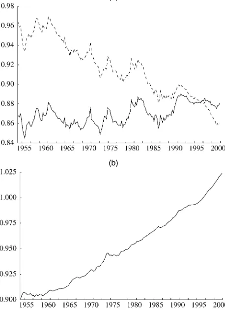
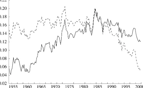
Of course, an empirical implementation of (13) will re-sult in a reasonable approximation to the correct underlying relationship only if (9) itself provides a reasonable empirical approximation. As is evident from Figure 1(a), however, the proposition that real nondurables and services consump-tion,Ctnd, represents a stable fraction of overall real consump-tion outlays,Ct, is clearly rejected in postwar U.S. data. Since the 1960s, this ratio has manifested a significant downward trend (a fact that has been noted in a number of previous em-pirical studies of consumption behavior). This implies that the approximation errorǫt in (9) has trended up over time, which should in turn cause the regression errorutin (13) to trend down over time.
2.2 Our Approach
Figure 1 also allows us to identify the source of the long-term decline in the ratio ofCndt toCt. From Figure 1(a) it is appar-ent that the ratio of nominal expenditures on nondurables and services,Cndt , to total nominal consumption expenditures,Ct, has been relatively stable over the postwar period. In particu-lar, although the nominal ratio may exhibit a very slight upward trend, any such trend is far less pronounced than the downward trend in the real ratio. Thus the significant disparity between the long-run growth rates of real expenditures on durable goods and real consumption of nondurables and services stems almost entirely from a large and ongoing decline in the relative price of durable goods. This trend—illustrated in Figure 1(b)—is part of a broader pattern in which prices for producers’ durable equip-ment have also been declining relative to prices for other goods and services, and is the result of productivity growth for the durable goods sector significantly outpacing that for the rest of the economy. (See Whelan 2003 for a more detailed discussion of the relative price shifts associated with sectoral differences in productivity growth.)
Figure 1 therefore indicates that an approximation like
Ct=γCndt +ηt (14)
(a)
(b)
Figure 1. Ratios of Quantities and Prices. (a) Ratio of consumption of nondurables and services to total consumption outlays [ , nominal data; , real data (1996 dollars)]; (b) ratio of nondurables and services price index to total consumption price index.
(whereηt denotes a mean-0—and probably heteroscedastic— approximation error) will provide a far more accurate descrip-tion of the data than (9). Indeed, over the sample period shown in the figure, the average absolute value of the approximation error for the relationship that assumes a stable real ratio [see (9)] is more than four times larger than the average absolute approx-imation error that obtains if a stable nominal ratio is assumed instead [as in (14)].
In addition, it is worth noting that this long-run relationship between nominal expenditures on durables and nominal expen-ditures on nondurables and services is also consistent with a Cobb–Douglas formulation of preferences whereby consumers maximize a lifetime utility function of the form
Et
∞
k=0
1 1+ρ
k
(Dt+k)α1(Cndt+k)
α2
. (15)
Moreover, if we retain the assumption that the market rate of interest is the same as the household discount rate, then we can use a first-order approximation to the household’s optimality condition to replace the martingale equation for total consump-tion with a martingale equaconsump-tion for consumpconsump-tion of nondurables and services,
EtCndt+1=Cndt . (16) These considerations suggest that we should seek to reformu-late the PIH under the alternative hypothesis of a stable long-run relationship between nominal expenditures on nondurable
goods and services and total nominal consumption outlays. It turns out that doing this is straightforward. Starting with (14), we can rewrite the nominal budget constraint, (1), as
At+1=(1+it+1)[At+Yt−γCndt −ηt]. (17) This equation can be reexpressed in terms of real consumption of nondurables and services by dividing through with the defla-tor for this series,Pndt+1,
Andt+1=(1+rtnd+1)[Andt +Ytnd−γCndt −ηt]. (18) In this form, the budget constraint involves real labor income, real financial wealth, and real interest rates, where in this case all real variables are defined relative to the deflator for non-durables and services,
The reformulated intertemporal budget constraint is ∞ and finally, using (16), the new structural solution for the PIH can be written as Hence the predictions of the PIH can again be reformulated us-ing a scaled version of real nondurables and services consump-tion, but this time using new measures of real labor income, financial wealth, and interest rates constructed by deflating with the price index for nondurables and services. In addition, this new formulation of the theory implies an alternative “wealth effect regression” of the form
γCndt
Because these derivations are based on (14), which is em-pirically much more accurate, the approximation errors in the resulting consumption relationships will be much smaller and hence less likely to present a major obstacle to tests of the un-derlying theory.
3. ESTIMATING THE WEALTH EFFECT
We have demonstrated that the methodology traditionally used in constructing structural tests of the PIH introduces sig-nificant measurement error in practice, and have proposed a simple alternative approach under which this error will be much smaller. We now explore how inferences about consumption be-havior are affected by using this alternative methodology. In our first example, we consider the PIH’s prediction of a long-run relationship between the ratio of consumption to labor income
and the ratio of financial wealth to labor income. Empirical esti-mates of the “cents-on-the-dollar” effect or marginal propensity to consume implied by this relationship are commonly cited, and these estimates play an important role in macroeconomic forecasting and policy analysis.
Our preceding analysis suggests, however, that the tradi-tional econometric consumption functions on which these es-timates are based contain a large and trending approximation error. As a result, we can make a number of predictions as to what we should expect from empirical implementations of these two approaches. First, the substantially larger measurement er-ror that obtains under the traditional formulation implies that the traditional version of the model should have a poorer fit. Second, our analysis suggests that the traditional approach con-tains a measurement error term that trends downward over time. Because the wealth-to-income ratio has, on balance, moved up-ward over our sample, there will be a negative correlation be-tween the wealth variable and an important component of the error term. Thus one would expect the traditional approach to produce smaller, downward-biased ordinary least squares es-timates of the wealth effect relative to our preferred method. Finally, one would also expect the traditional approach’s trend-ing error to yield coefficient estimates that exhibit more para-meter instability.
Taken together, then, a priori reasoning suggests that our pre-ferred methodology should yield a better-fitting regression with larger and more stable estimates of the wealth effect. It turns out that each of these predictions is verified by the data.
3.1 Implementing the Wealth Effect Models
Before describing our wealth effect regressions, we briefly mention one detail concerning the models’ implementation. To bring (13) and (22) to the data, we first need estimates of the scaling parametersθ andγ. We estimate these parameters as the ratio of mean total consumption to mean nondurables and services consumption, where real values of both series are used for θ and nominal values are used forγ. Hence we measure
θandγ as
Because this procedure involves replacing a true parameter with an econometric estimate, we might be concerned about the validity of standard statistical inference in some contexts (particularly whereθˆorγˆ is used to construct an independent variable in a regression). However, for our preferred method (based on nominal values), formal statistical tests indicate that the linear combinationCt− ˆγCtnd is stationary [a finding con-sistent with the informal visual evidence provided by Fig. 1(a)]. Hence we can treat this estimate of the scaling parameter as su-perconsistent, which in turn implies that it can be treated as known rather than generated. As might be expected, however, the same is not true for the traditional method. One fails to re-ject the hypothesis of no cointegration for the corresponding
linear combination of real variables. In what follows, we report the usual standard errors for this case, but note that the potential inaccuracy of these statistics represents another potential prob-lem with the traditional method.
3.2 Empirical Results
We now examine how our methodology affects various fea-tures of the empirical wealth effect regressions, including their fit, point estimates, and stability over time.
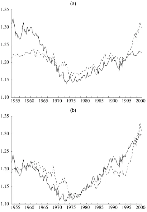
3.2.1 Fit. To confirm our conjecture that the relationship based on the traditional approach will have a poorer fit be-cause of larger approximation errors, Figure 2 plots fitted values from our two wealth effect regressions against their respec-tive dependent variables. Figure 2(a) plots the results based on the traditional deflation technique, whereas Figure 2(b) gives the values obtained when our preferred deflation proce-dure is used. (The sample period for these regressions extends from 1954:Q1 to 2000:Q4.) The figure shows that the estimated consumption–wealth relationship fits much worse when the tra-ditional deflation procedure is used; the regression based on our deflation method has anR¯2of .71, compared with anR¯2of .36 under the traditional deflation procedure.
Of course, this poor fit would not necessarily cause a re-searcher to reject the permanent income hypothesis. Neverthe-less, it may yield a somewhat misleading picture of what must
(a)
(b)
Figure 2. Ratio of Consumption to Labor Income. Actual ( ) and fitted ( ) values from a regression of the consumption–income ratio on the wealth–income ratio using (a) the traditional deflation method and (b) our deflation method.
be going on if the model is, in fact, correct. For instance, we could attempt to reconcile the PIH with the poor fit shown in Figure 2(a) by positing a specific pattern of expectations con-cerning future labor income growth over this period; as noted, the theory predicts that these expectations are a component of the regression’s residual. However, our analysis suggests a much simpler explanation related to the presence of trending measurement error.
3.2.2 Estimates of the Wealth Effect. Our predictions con-cerning the effect of the traditional deflation procedure on the size of the estimated wealth effect are also confirmed by these regressions. As reported in Table 1, when we fit (22), which uses our preferred deflation methodology, we obtain an esti-mate of α1=.070 (with a standard error of .005), compared with a point estimate of .050 (standard error of .016) under the traditional deflation method.
Our estimate of a 7 cents per dollar wealth effect is notewor-thy because it is substantially larger than the average estimate reported using the traditional deflation methodology. Other au-thors have tended to report estimates of the wealth effect in the 3- to 4-cent range; indeed, Poterba’s (2000) survey of these results notes that the upper bound of previously reported esti-mates appears to be 5 cents on the dollar.
As we have noted, the PIH implies that the error term in this regression is related to expectations of future growth in labor income. We therefore checked whether these results are robust to the addition of variables that may proxy for such expecta-tions by adding the contemporaneous value of real labor income growth and four of its lags (where real labor income is defined relative to the total consumption deflator for the traditional ap-proach and relative to the price index for consumer nondurables and services for our approach). Wealth effect estimates from these augmented models (not shown) are basically identical to those from our baseline specifications. Interestingly, however, we find that the additional labor income variables improve the fit of the regression under our estimation method but have no significant effect in the traditional wealth effect regression.
3.2.3 Stability. Our predictions concerning the effect of the traditional deflation method on parameter stability also turn out to match the data. Specifically, estimates of the propen-sity to consume out of wealth using our preferred method turn out to be relatively stable across different subsamples,
Table 1. Results From Wealth Effect Regressions
Sample period α1 R¯2
Using traditional deflation
1954:1–2000:4 .050 .363
(.016)
1954:1–1975:4 .125 .714
(.015)
1976:1–2000:4 .032 .781
(.005) Using our deflation procedure
1954:1–2000:4 .070 .711
(.005)
1954:1–1975:4 .081 .667
(.012)
1976:1–2000:4 .067 .849
(.008)
NOTE: Newey–West HAC standard errors are in parentheses; allα1andβ1estimates are significant at the 1% level. See the text for additional details.
whereas estimates based on the traditional method are more sensitive. Inspection of Figure 2(b) shows that the predicted consumption–income ratio from the regression using our defla-tion procedure is systematically too high up to 1975, and then generally too low thereafter. However, reestimating this equa-tion over each subsample gives estimates of the propensity to consume out of wealth of .081 for the early period and .067 for the later period—figures that are not too far apart. In contrast, estimates obtained under the traditional deflation technique im-ply propensities to consume out of wealth that are very differ-ent over these subsamples—.125 over the early period and .032 over the later period. (Note that this finding is also robust to the addition of contemporaneous and lagged real labor income growth to the baseline regression.)
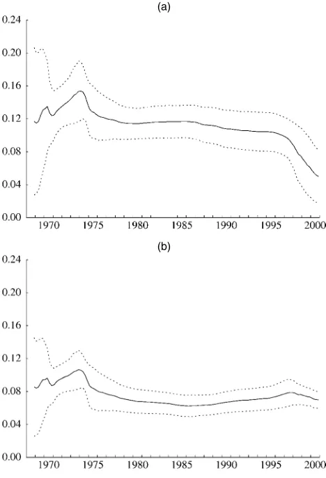
Another way to demonstrate the relative stability of the wealth effect produced by our approach involves plotting recur-sive estimates, which are obtained from a sequence of regres-sions that add an observation at each step. Figure 3(b) shows that the recursive estimates produced by our method settle down quickly and then remain within a narrow band that is close to the full-sample estimate. In contrast, Figure 3(a) indicates that the estimates produced by the traditional approach mani-fest an almost monotonic decline from the mid-1970s onward. This finding of an unstable, declining wealth effect has
previ-(a)
(b)
Figure 3. Recursive Regression Estimates of the Wealth Effect. (a) Estimates obtained using the traditional deflation method (based on real ratios); (b) estimates obtained using our deflation method (based on nominal ratios). Dotted lines represent 95% confidence intervals.
ously been reported by other authors who used the traditional deflation methodology (e.g., Ludvigson and Steindel 1999); our results suggest that this instability may in part be merely an ar-tifact of a trending approximation error, which drives a wedge between the true underlying relationship and its empirical coun-terpart.
Finally, we note in passing that formal structural change tests, such as the Quandt likelihood ratio (or sup-F) test, formally re-ject the hypothesis of no change over time in the wealth effect coefficient even under our methodology. That said, our point is not that this coefficient is completely stable, but rather that any changes over time appear to be relatively small. More-over, it is clearly the case that our view of the size of these changes will be profoundly affected by our choice of deflation methodology.
4. SAVING FOR A RAINY DAY?
The foregoing results demonstrate that the approximation er-rors induced by the traditional approach to deflating income and wealth can seriously affect the interpretation of one type of relationship implied by the PIH. Left unanswered, of course, is whether the hypothesis itself is valid. We now consider how tests of a basic implication of the PIH are affected by the choice of deflation procedure. Specifically, we examine the well-known prediction discussed by Campbell (1987) and Campbell and Deaton (1989) that saving out of disposable in-come should Granger cause future declines in labor inin-come. If we define saving as
St= r
1+rAt+Yt−Ct, (25) then it can be shown (see Campbell and Deaton 1989) that the structural version of the PIH [see (8)] implies the following ap-proximate relation:
St Yt
≈ −
∞
k=1
βkEtlogYt+k+κ, (26)
whereκdenotes a constant of linearization. In this expression, the discount factorβ equals 11++µr, whereµis the expected log-difference of future values ofYt. [Note that combining (26) with the definition of saving yields (12) from Sec. 2.]
Equation (26)—the so-called “saving for a rainy day” equa-tion—implies that the saving rate (defined as the ratio of saving to labor income) should be negatively correlated with future growth in real labor income. Besides examining the effect of the two deflation methods on empirical tests of this proposi-tion, we also consider two different approaches to testing this hypothesis based on different ways of measuring 1+rrAt(which corresponds to the real capital income received by consumers).
4.1 Tests Using NIPA Capital Income
Both Campbell (1987) and Campbell and Deaton (1989) equated1+rrAtwith personal capital income as measured in the
National Income and Product Accounts (NIPAs); as a result, the disposable income series used in both of these studies was identical to the NIPA definition. Here we follow these authors in using this income measure to compute saving and examine whether the lagged ratio of saving to labor income (the “saving rate”) helps forecast the log-difference of real labor income in equations like
As Campbell and Deaton have emphasized, as long as house-holds have more information about their future labor income than what is present in lagged labor income growth, then the PIH predicts that the saving rate will play an empirical role in helping to forecast changes in labor income.
Under the traditional deflation procedure, the Campbell– Deaton saving rate is measured as
St
whereYtd is real NIPA disposable income andYt is real labor income, both defined relative to the total consumption deflator. Again,θ is our estimate of the “real” scaling factor from (9), andCndt is real nondurables and services consumption. We use these definitions of the saving rate and real labor income to fit versions of (27) that include various lags of each variable; esti-mation runs from 1954:Q1 to 2000:Q4.
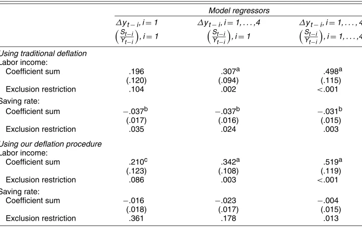
The upper part of Table 2 presents the estimated coefficients on lagged labor income growth and the lagged saving rate (along with thepvalues from tests of the exclusion restrictions) that we obtain from this exercise. Starting with the results in the first column (which are from the specifications with one lag of labor income growth and one lag of the saving rate), we see that the saving rate enters the regression for labor income growth
with the negative coefficient that the theory predicts; moreover, the coefficient is statistically significant at close to the 1% level. Similar results obtain when we allow for four lags of labor in-come growth (the second column), as well as when we include four lags of labor income growth and four lags of the saving rate in the regression (the third column); in each case, the coef-ficient (or sum of coefcoef-ficients) on the saving rate is negative and highly statistically significant. Hence the results obtained using the traditional deflation method confirm the original findings of Campbell and Deaton that higher saving appears to anticipate slower labor income growth.
This conclusion changes significantly when we use our pre-ferred deflation method. Here the saving rate is defined as
St inal consumption of nondurables and services, Yt is nominal labor income, andγis our estimate of the “nominal” scale fac-tor in (14). (Note that this is equivalent to deflating all nom-inal variables by the price index for nondurable goods and services consumption.) Results from these models are summa-rized in the lower part of the table. For the regressions with one lag of the saving rate (reported in columns one and two), we find that the point estimates of the coefficient on the sav-ing rate, although negative, are smaller and no longer statisti-cally significant. As a result, these specifications provide much less evidence that saving Granger causes income growth. When we allow four lags of each variable to enter the regression (column three), we find somewhat stronger evidence of Granger causality in the sense that the coefficients on the four lags of the saving rate are jointly significant at roughly the 1% level. How-ever, the coefficients on the saving rate essentially sum to 0 (and this sum is statistically insignificant), implying that a higher
Table 2. Results From Rainy Day Saving Equations
Model regressors
Coefficient sum .196 .307a .498a
(.120) (.094) (.115)
Exclusion restriction .104 .002 <.001 Saving rate:
Coefficient sum −.037b −.037b −.031b
(.017) (.016) (.015)
Exclusion restriction .035 .024 .003
Using our deflation procedure
Labor income:
Coefficient sum .210c .342a .519a
(.123) (.108) (.119)
Exclusion restriction .086 .003 <.001 Saving rate:
Coefficient sum −.016 −.023 −.004
(.018) (.017) (.015)
Exclusion restriction .361 .178 .013
NOTE: Newey–West HAC standard errors are in parentheses; a, b, and c denote significance at the 1%, 5%, and 10% levels. “Exclusion restriction” gives thepvalue from anF-test that lags of given variable can be excluded from the model. Regressions include indicated number of lags of saving rate and log-differenced labor income; dependent variable in all equations is log-differenced labor income. See the text for additional details.
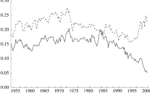
Figure 4. Two Measures of the Saving Rate ( traditional deflation; alternative deflation).
level of saving does not tend to signal future lower labor in-come growth. It is difficult to argue that this result provides strong support for the PIH; in any case, these results stand in sharp contrast to those obtained using the traditional deflation procedure.
Another interesting result (not reported in the table) is that the preferred deflation procedure actually does suggest that in-creased rates of saving anticipate lower labor income growth when the forecasting regressions are estimated through 1984 (the end of the sample considered by Campbell and Deaton). Apparently, therefore, it is the introduction of the late 1980s and 1990s that weakens the evidence for Granger causality. Fig-ure 4, which plots the saving rates obtained under the alternative and traditional deflation procedures, helps explain why. After the mid-1980s, the saving rate generated by our alternative pro-cedure falls to very low levels, mirroring, for example, the sub-stantial decline in the official NIPA saving rate (which is also calculated as a ratio of nominal series). In contrast, the saving rate calculated using the traditional deflation method declines by a much smaller amount. Labor income growth did, in fact, pick up in the 1990s, but not by nearly as much as would be implied by the saving measure derived under our deflation pro-cedure. Hence the traditional method’s measure of the saving rate appears to do a better job forecasting real labor income.
Of course, this latter saving rate remains quite high during the 1990s for an unsatisfactory reason—namely that, relative to the theoretically correct measure of saving that would forecast labor income growth if the PIH were correct, this series con-tains an upward-trending approximation error associated with the traditional treatment of durable goods. Put differently, the fact that nominal nondurables and services consumption has re-mained a roughly stable share of total nominal consumption outlays implies that declining prices of durable goods have resulted in a proportional increase in real durables expendi-tures. When we apply the traditional deflation technique, these declines in durable goods prices boost real income; however, this additional real income is not measured as being spent on real consumption (defined as scaled-up real nondurables and services expenditures). As a result, under the traditional defla-tion method, the measured saving rate is propped up over the 1990s.
4.2 Tests Using Regression-Based Measures of Capital Income
One possible explanation for our failure to find evidence of Granger causality from saving to labor income growth could be that the NIPA capital income series provides a poor proxy for the appropriate theoretical concept of real capital in-come, 1+rrAt. There are several reasons why this might be so. First, the correct theoretical rate of return on wealth should in-clude capital gains; however, the national accounts measure of capital income includes only flow payments such as dividends and interest. Moreover, even if the current-period flow of nom-inal capital income in the NIPAs were to correspond exactly to 1+iiAt (whereidenotes the nominal interest rate), we would not recover the desired real capital income concept, 1+rrAt, by deflating the NIPA measure by a price index. Rather, we must subtract a term equal to 1π+iAt—whereπis the average (antici-pated) inflation rate—from the deflated nominal capital income as well. In general, this provides a rationale for adjusting saving measures for the effect of inflation (cf. Wilcox 1991).
Finally, the formulation of the rainy day equation that we have been working with has been derived from the assumption that nondurables and services consumption follows a martin-gale. But this result relies on the very restrictive assumption that the rate of time preference equals the market rate of inter-est. Once we weaken this assumption, we can approximate the first-order condition for optimal consumption of nondurables and consumption as
EtCtnd+1=
1+ρ
1+rnd
Ctnd. (30)
Combining this with our expression for the intertemporal bud-get constraint [see (10)], we can derive the following approxi-mate relationship:
1+rnd r−ρ
Andt
Ytnd −γ Ctnd
Ytnd ≈ −
∞
k=1
βkEtlogYtnd+k+k. (31)
In other words, once we allow for the possibility of trending consumption, we can still obtain a long-run linear relationship between the scaled consumption–income ratio and the wealth– income ratio, with deviations from this relationship being re-lated to expectations about future labor income growth.
These considerations imply that, strictly speaking, we should not expect standard saving measures to forecast labor income growth even if the PIH is true. However, a prediction common to both versions of the PIH that we have derived is that the errors from a regression of the scaled consumption–income ra-tio on the wealth–income rara-tio should forecast labor income changes. This regression-based measure of the “saving rate” can therefore be used in the forecasting regression [see (27)]. Figure 5 plots the regression-based measure together with the NIPA-based saving rate that we obtained earlier under our pre-ferred deflation procedure. As expected, the higher capital in-come imputed from the regression-based approach keeps this measure of the saving rate from declining sharply during the 1990s; indeed, the regression-based measure actually rises over the latter half of the decade.
We examined whether this variant of the saving rate is better able to forecast labor income growth by using it to repeat the
Figure 5. Saving Rate With Regression-Based Capital Income Mea-surement ( alternative deflation method; with regression-based capital income).
analysis of Section 4.1; the relevant results are summarized in Table 3. Perhaps surprisingly, we once again are unable to find strong evidence that the saving rate Granger causes labor in-come growth; as the table indicates, we fail to reject the hypoth-esis that the regression-based saving rate can be excluded from the regressions for labor income growth at conventional signif-icance levels. In addition, the sign of the coefficient (or sum of coefficients) on the saving rate is positive, not negative as the theory would predict. Evidently, then, some additional exten-sion is needed to salvage this prediction of the PIH.
5. COINTEGRATION AMONG CONSUMPTION, WEALTH, AND INCOME
Up to now, we have assumed that asset returns are determin-istic and fixed. Lettau and Ludvigson (2001) derived some long-run restrictions on the joint behavior of consumption, assets, and income in a model with time-varying asset returns. They used a methodology proposed by Campbell and Mankiw (1989) to construct a log-linear approximation to the consumer budget constraint [our (5)]. Under various assumptions about the sta-tionarity of consumption growth and the returns on human and nonhuman wealth, they demonstrated that the budget constraint implies a cointegrating relationship between log consumption,
log assets, and log labor income,
ct−αat−(1−α)yt∼I(0), (32) where the cointegrating parameter αis related to the average share of nonhuman wealthA(assets) in total wealth, with lower-case letters used to denote log quantities.
Lettau and Ludvigson did not directly test this cointegration relationship. Instead, in keeping with the traditional consump-tion literature—and despite the fact that (32) is based not on a behavioral relationship (such as a consumption Euler equa-tion), but only on an aggregate budget constraint—they re-placed the log of total real consumption ct with a measure of real nondurables and services consumption cndt . They then tested whethercndt is cointegrated with real assets and real labor income (where these latter measures are constructed by deflat-ing nominal assets and labor income with the price index for total consumption). They presented test results supporting the hypothesis of a cointegrating relation amongcndt ,at, andytand demonstrated that the resulting cointegrating residual predicts future asset growth—a finding with obvious important implica-tions for financial economics.
In a critique of Lettau and Ludvigson’s procedure, Rudd and Whelan (in press) pointed out that the hypothesis of a cointe-grating relation amongcndt ,at, andytcan be justified only if the logs of total real consumptionctand nondurables and services consumptioncndt are themselves cointegrated. As we might ex-pect given our preceding analysis, there is little theoretical or empirical reason to expect these series to be cointegrated, and indeed Rudd and Whelan demonstrated that standard tests fail to reject the hypothesis of no cointegration between these vari-ables. (Note that Lettau and Ludvigson conducted their analysis in logs and included shoes and clothing in their definition of durable goods; however, as Rudd and Whelan demonstrated, the ratio of log real total consumption to Lettau and Ludvigson’s measure of log real nondurables and services consumption also manifests a pronounced upward trend in postwar U.S. data.) Furthermore, Rudd and Whelan showed that when one di-rectly tests the cointegrating hypothesis associated with (32)— in other words, when one uses total real consumption in lieu of cndt —then statistical tests fail to reject the hypothesis of no cointegration, suggesting that any predictive relationship based on an estimated linear combination of these variables is ques-tionable.
Table 3. Rainy Day Saving Equations, Regression-Based Capital Income
Model regressors
∆yt−i, i=1 ∆yt−i, i=1, . . . ,4 ∆yt−i, i=1, . . . , 4 S
t−i
Yt−i , i=1
S
t−i
Yt−i , i=1
S
t−i
Yt−i , i=1, . . . ,4
Labor income:
Coefficient sum .171 .247a .252a
(.136) (.140) (.143)
Exclusion restriction .209 .329 .380
Saving rate:
Coefficient sum .029 .020 .019
(.028) (.029) (.029)
Exclusion restriction .311 .486 .801
NOTE: Newey–West HAC standard errors are in parentheses; a denotes significance at the 10% level. “Exclusion restriction” gives the
pvalue from anF-test that lags of given variable can be excluded from the model. Regressions include indicated number of lags of saving rate and log-differenced labor income; dependent variable in all equations is log-differenced labor income. See the text for additional details.
These results provide additional support for Brennan and Xia’s (2005) claim that the relationship between asset growth and the residual from Lettau and Ludvigson’s (cndt ,at,yt) regression may be spurious. Brennan and Xia showed that re-placing consumption with a simple time trend yields a “coin-tegrating residual” that still apparently forecasts asset growth. Lettau and Ludvigson (2005) responded to this critique by ar-guing that both economic theory and empirical tests suggest a cointegrating relationship between cndt ,at, andyt. However, the theoretical basis for such a relationship is, in fact, relatively weak, and once one examines an empirical relationship that is actually consistent with theory, one obtains evidence for coin-tegration that is also much weaker.
Although a full consideration of the arguments in this debate would take us too far afield, we view Rudd and Whelan’s re-sults as underscoring this article’s basic message: Variables that are linked by a budget constraint must be transformed into real equivalents in a manner that respects and preserves the budget constraint’s underlying nominal relationship (e.g., by deflating both sides of the constraint with the same price index).
6. CONCLUSIONS
This article has examined the well-known problem of how to test theories of consumer behavior when consumption ex-penditures include durable goods purchases. Specifically, we have presented theoretical and empirical arguments for relating real consumption of nondurable goods and services to measures of real income and wealth defined relative to a price index for nondurables and services consumption. This contrasts with the usual procedure of deflating income and wealth with a price in-dex for total consumption. In two empirical exercises, we have demonstrated that this choice of deflation method can signifi-cantly affect the interpretation of observed consumption behav-ior as well as the results obtained from standard tests of the predictions of the permanent income hypothesis.
Beyond the substantive results relating to tests of consumer behavior, a more general lesson that we take from these findings is that macroeconomists may need to be somewhat more care-ful regarding their treatment of “real” variables. It is perhaps understandable that economists, who are schooled in the dic-tum that real variables “control for changes in the price level,” might conclude that deflation by a broad-based price index is always the appropriate way to construct a real income, output, or wealth series. However, our analysis shows that this practice can sometimes result in a poor empirical approximation to the underlying theoretical relationship that we seek to capture.
ACKNOWLEDGMENTS
The authors thank the associate editor and three anonymous referees for useful comments on an earlier draft of the manu-script. The views expressed are the authors’ own and do not necessarily reflect the views of the Board of Governors, the staff of the Federal Reserve System, or the Central Bank of Ireland.
APPENDIX: DATA SOURCES AND DEFINITIONS
Note that the consumption, wealth, and income variables used in the wealth effect and rainy day regressions are ex-pressed in per-capita terms using the population measure de-scribed herein.
Consumption Expenditures. Total personal consumption expenditure is taken from NIPA data. Consumption of non-durables and services is computed by combining NIPA personal consumption expenditures on nondurable goods with NIPA per-sonal consumption expenditures on services. Real measures are combined using a Fisher chain-aggregation formula that repli-cates the procedure used by the Bureau of Economic Analysis in producing the NIPAs.
Consumption Prices. Price indexes are defined as implicit deflators, that is, as ratios of nominal series to corresponding real series.
Wealth. All data are taken from the Flow of Funds Ac-counts of the Board of Governors of the Federal Reserve Sys-tem, table B.100. Wealth is defined as household net worth less stocks of consumer durable goods. Flow of Funds wealth mea-sures are expressed on an end-of-period basis; we therefore as-sociate the t−1 value of the data with period t wealth (i.e., withAt) to obtain a start-of-period measure.
Disposable Income. NIPA disposable income (table 2.1). Following Blinder and Deaton (1985), we reduce disposable in-come in 1975:Q2 by $32.5 billion (at an annual rate) to remove the effect of the 1975 tax rebate from measured income.
Labor Income. We define labor income as wage and salary disbursements plus transfers to persons plus other labor income minus personal contributions for social insurance minus labor taxes. Labor taxes are defined by imputing a share of personal tax and nontax payments to labor income, with the share calcu-lated as the ratio of wage and salary disbursements to the sum of wage and salary disbursements, proprietors’ income, and rental, dividend, and interest income. Note that personal tax and non-tax payments are adjusted for the effect of the 1975 non-tax rebate. (All series are taken from NIPA table 2.1.)
The definition of labor income used in this article differs from the measure used by Blinder and Deaton (1985), which was in turn used by Campbell (1987) and Campbell and Deaton (1989). We redid the analysis of Section 5 using two variants of an updated Blinder–Deaton income series and found that the substantive conclusions were unaffected by using these alterna-tive measures.
Population. These are the population figures from NIPA ta-ble 2.1. (Note that this is the population measure used by the Bureau of Economic Analysis to compute official per-capita in-come and consumption data.)
[Received June 2004. Revised July 2005.]
REFERENCES
Blinder, A. S., and Deaton, A. (1985), “The Time Series Consumption Function Revisited,”Brookings Papers on Economic Activity, 2, 465–521.
Brennan, M. J., and Xia, Y. (2005), “tay’s as Good ascay,”Finance Research Letters, 2, 1–14.
Campbell, J. Y. (1987), “Does Saving Anticipate Declining Labor Income? An Alternative Test of the Permanent Income Hypothesis,”Econometrica, 55, 1249–1273.
Campbell, J. Y., and Deaton, A. (1989), “Why Is Consumption so Smooth?” Review of Economic Studies, 56, 357–374.
Campbell, J. Y., and Mankiw, N. G. (1989), “Consumption, Income, and Inter-est Rates: Reinterpreting the Time Series Evidence,”NBER Macroeconomics Annual 1989, 4, 185–216.
Galí, J. (1990), “Finite Horizons, Life-Cycle Savings, and Time-Series Evi-dence on Consumption,”Journal of Monetary Economics, 26, 433–452.
Hall, R. E. (1978), “Stochastic Implications of the Life Cycle-Permanent In-come Hypothesis: Theory and Evidence,”Journal of Political Economy, 86, 971–987.
Lettau, M., and Ludvigson, S. (2001), “Consumption, Aggregate Wealth, and Expected Stock Returns,”Journal of Finance, 56, 815–849.
(2005), “tay’s as Good ascay: Reply,”Finance Research Letters, 2, 15–22.
Ludvigson, S., and Steindel, C. (1999), “How Important Is the Stock Market Effect on Consumption?”Federal Reserve Bank of New York Policy Review, July, 29–51.
Poterba, J. (2000), “Stock Market Wealth and Consumption,”Journal of Eco-nomic Perspectives, 14, 99–118.
Rudd, J., and Whelan, K. (in press), “Empirical Proxies for the Consumption– Wealth Ratio,”Review of Economic Dynamics, in press.
Whelan, K. (2003), “A Two-Sector Approach to Modeling U.S. NIPA Data,” Journal of Money, Credit, and Banking, 35, 627–656.
Wilcox, D. W. (1991), “Household Spending and Saving: Measurement, Trends, and Analysis,”Federal Reserve Bulletin, January, 1–17.