Full Terms & Conditions of access and use can be found at
http://www.tandfonline.com/action/journalInformation?journalCode=ubes20
Download by: [Universitas Maritim Raja Ali Haji] Date: 13 January 2016, At: 00:47
Journal of Business & Economic Statistics
ISSN: 0735-0015 (Print) 1537-2707 (Online) Journal homepage: http://www.tandfonline.com/loi/ubes20
Measuring and Decomposing Productivity Change
Scott E Atkinson, Christopher Cornwell & Olaf Honerkamp
To cite this article: Scott E Atkinson, Christopher Cornwell & Olaf Honerkamp (2003)
Measuring and Decomposing Productivity Change, Journal of Business & Economic Statistics, 21:2, 284-294, DOI: 10.1198/073500103288618963
To link to this article: http://dx.doi.org/10.1198/073500103288618963
Published online: 24 Jan 2012.
Submit your article to this journal
Article views: 93
View related articles
Measuring and Decomposing Productivity
Change: Stochastic Distance Function
Estimation Versus Data Envelopment Analysis
Scott E.
Atkinson
, Christopher
Cornwell
, Olaf
Honerkamp
Department of Economics, University of Georgia, Athens, GA 30602
(atknsn@terry.uga.edu) (cornwl@terry.uga.edu) (olaf.honerkamp@mirant.com)
Measuring productivity change with Malmquist indices has become common practice, because they are easily computed using nonparametric programming techniques and can be readily decomposed into technical and efciency change. However, this approach is nonstochastic and requires a constant returns to scale assumption to construct the reference technology. We propose estimating productivity change using a stochastic input distance frontier, imposing no restrictions on returns to scale. We derive the analogous decomposition of productivity change and develop a generalized method of moments strategy in which outputs or inputs may be endogenous. We compare two methods in an application to electric utilities.
KEY WORDS: Distance function; Efciency change; Generalized method of moments; Malmquist indices; Panel data; Productivity change; Technical change.
1. INTRODUCTION
Caves, Christensen, and Diewert (1982) (hereafter CCD) developed Malmquist output and input productivity change (PC) indices for multiple-input, multiple-output technologies that are valid for any returns to scale. The output- (input-) oriented index is based on an output (input) distance func-tion and reects changes in maximum output (minimum input requirements) given inputs (outputs). CCD stated that unless some functional form is specied for a parametric produc-tion frontier, these indices cannot be computed. As an index number alternative, CCD proved that for translog (TL) struc-tures of production, a T ¨ornqvist output (input) index can be constructed as the geometric mean of two Malmquist out-put (inout-put) indices using data on prices and quantities, with-out knowledge of the TL parameters dening the produc-tion frontier.
F¨are, Grosskopf, Norris, and Zhang (1994) (hereafter FGNZ) extended the work CCD in two important ways. First, FGNZ showed how to compute Malmquist indices relative to a nonparametric specication of the production frontier. They did so by using the nonparametric, linear program-ming techniques of data envelopment analysis (DEA) to t distance functions to data on input and output quantities. They directly calculated PC as the geometric mean of two Malmquist productivity indices, without price data and with-out using a TL functional form. Second, FGNZ generalized the CCD approach by decomposing the PC index into techni-cal change (TC) (frontier shifts) and efciency change (EC) (movements toward the frontier). However, whereas FGNZ’s approach is nonparametric, it imposes a constant returns to scale (CRS) restriction on the frontier technology. FGNZ used a variable returns to scale (VRS) technology only for the pur-pose of further decomposing EC. Ray and Desli (1997) dis-agreed with FGNZ on roles of the VRS and CRS frontiers in thedecompositionof PC indices and proposed an alterna-tive. Nevertheless, Ray and Desli concurred with FGNZ on the necessity of the CRS assumption in computing the overall PC index. These issues do not arise in our econometric approach.
A stochastic alternative that assumes a exible functional form approximation to the frontier was provided by Chris-tensen, Caves, and Swanson (1981) (henceforth CCS), who estimated a TL cost function. They exploited the dual relation-ship between a transformation function and a cost function to show that an input-oriented distance measure of PC can be expressed as the negative of the time rate of change in the cost function, which is TC. This result allowed them to com-pute PC as minus the time derivative of their estimated TL cost function, rather than having to estimate the transforma-tion functransforma-tion. However, CCS imposed the restrictive assump-tion that all rms are technically efcient, so that EC is zero. Further, they did not develop the methodology to directly esti-mate the input distance function, which is dual to their cost function.
Our purpose in this article is to combine and extend the best elements of the CCS and FGNZ approaches within a dual-input distance function framework. First, we show that by imposing linear homogeneity in input quantities on the general transformation function used by CCS, we obtain an input dis-tance function, which is dual to a cost function. Next, we gen-eralize the CCS approach to incorporate time-varying techni-cal inefciency by postulating a frontier distance function. We use this framework to decompose PC analogously to FGNZ. In particular, we establish that TC equals the time derivative of the log of the frontier distance function, and that PC can be expressed as the sum of TC and EC. To our knowledge, the analog to the FGNZ decomposition has not been devel-oped for a parametric stochastic distance frontier. Finally, we propose a generalized method of moments (GMM) strategy for estimating such a model that does not restrict outputs or inputs to be exogenous.
©2003 American Statistical Association Journal of Business & Economic Statistics April 2003, Vol. 21, No. 2 DOI 10.1198/073500103288618963
284
Importantly, our econometric approach enables specication tests of the underlying moment conditions, as well as tests of the usual parametric hypotheses. In general, this is not pos-sible using DEA. Moreover, because DEA is nonstochastic, all departures from the reference technology are attributed to inefciency, which can lead to implausibly wild uctuations in PC, EC, and TC from period to period. By adopting a para-metric model and accounting for noise, we should nd less volatility in the temporal patterns of PC and its components.
To examine the implications of these different methodolo-gies, we apply them to a newly updated panel of 43 U.S. electric utilities operating over the period 1961–1992. We con-trast DEA-based Malmquist indices of PC with those derived from the estimated TL frontier distance function. We nd that the two approaches yield positive and generally similar annual rates of PC, but conict more sharply in terms of the relative importance of TC to EC in explaining overall growth. We cal-culate an average annual rate of PC of 1.04% using DEA, ver-sus .56% as derived from our estimated TL. However, with the estimated TL, all of the average productivity gain is attributed to TC, whereas with DEA there is a roughly equal balance between TC and EC. We also nd that the temporal patterns in PC, TC, and EC generated by the two approaches differ con-siderably, with much greater volatility exhibited in the DEA series. Qualitatively, these contrasts are robust to the choice of instruments. We conclude that the failure of DEA to account for noise is the most likely explanation for the differences in results. The assumption of CRS is a less likely causal factor, but its exact role is difcult to evaluate.
2. A MALMQUIST INPUT PRODUCTIVITY INDEX
Let the technology be described in terms of an input corre-spondence, ment set. Then, for a given rm, the input distance function is dened as the maximum scale factor necessary to placext on the boundary ofLt4
where theisubscript indicates an input distance function. Thus xt2Lt4yt5 if and only if Dit4yt1xt5¶1. This property is a consequence of assuming free disposability of inputs, that is, xt2Lt4yt51x tion is homogeneous of degree 1, nondecreasing, and quasi-concave in the inputs and is nonincreasing and quasi-quasi-concave in the outputs. The reciprocal ofDt
i is the input-oriented mea-sure of technical efciency, which is given by
£
Although a Malmquist PC index can be constructed relative to the technology in period t ortC1, we follow FGNZ and compute the geometric mean of the two indices. The empiri-cal Malmquist index is obtained using DEA, which involves solving a series of linear programming problems to calcu-late the distance functions (see FGNZ for details). Note, how-ever, that the formulas of FGNZ are based on the output distance function,Dt
o4yt1xt5. Rising productivity implies that the value of Dt
i4yt
C11
xtC15 is falling toward one relative to
Dt associate bigger with better in terms of productivity growth, we invert the formulas given by FGNZ. Thus values of PC, EC, and TC greater (less) than 1 indicate increased (decreased) productivity, increased (decreased) efciency, and technical progress (regress), respectively.
3. ESTIMATING PRODUCTIVITY CHANGE USING DISTANCE FUNCTIONS
3.1 General Form of the Stochastic Distance Function
Before proceeding further, we translate our previous expres-sion of the distance function, which is typical in the DEA lit-erature, into a notation more typical of an econometric model. Therefore, we dene
Ideally, a stochastic version of (4) would lead to a typical additive-error regression model. As F¨are and Primont (1996) demonstrated, such a model can be justied by appealing to the duality between the cost function, C4yft1pft1 t5, where pft is a vector of input prices, and the input distance func-tion. Let …ft be a random variable and g be a function of
…ft. Then, assuming that we can express the cost function £4y
ft1pft1 t1 g4…ft55as C4yft1pft1 t5g4…ft5(i.e., the cost func-tion has a multiplicative form), we can express the distance function,¤ holds only if xft is an element of the isoquant of the input requirement set. Deviations from 1, due to technical inef-ciency, are accommodated through the specication ofh4…ft5, so that the stochastic input distance function can be written as
1DDi4yft1xft1 t5h4…ft50 (6)
Then, after assuming functional forms for Di4yft1xft1 t5 and
h4…ft5, (6) can be estimated econometrically after imposing linear homogeneity in inputs.
3.2 Deriving and Decomposing Productivity Change
We now generalize the stochastic framework of CCS by deriving PC subject to technical inefciency measured from a frontier distance function, which allows the decomposition of PC into TC plus EC. Further, by solving the cost-minimization problem where the constraint is the input distance function, we obtain TCD ƒ¡lnC
¡t ²ƒ PC, which implies that PCD ƒ PCCEC. For simplicity, we temporarily suppress the f and t sub-scripts and write h4…ft5 as h4t5. Then, due to linear homo-geneity inx, (6) becomes
Di6y1 h4t5x1 t7DDi4y1xQ1 t5D11 (7)
Now multiply and divide the denominator of the middle term on the left side of (8) byxQn. Because an input distance function is dened as a common scalar contraction of inputs, we holdy constant (dyD0) and use a common scalar for xQ
4dlnxQ1=dtD¢ ¢ ¢DdlnxQN=dt5. These restrictions imply that one can factor the common scalar through the summation sign and obtain
Because the input distance function is linearly homogeneous in the inputs, the denominator of the left side of (9) can be written as Di4y1xQ1 t5. This same property allows us to expressDi4y1xQ1 t5as h4t5Di4y1x1 t5. On cancellation of h4t5 in numerator and denominator, we can express (9) as
¡Di4y1x1t5
Further, we can write the left side of (10) as
¡Di4y1x1t5
dt , we combine (11)–(13) to obtain
PCD¡lnDi4y1x1 t5
¡t C Ph4t5DTCCEC0 (13)
In addition, we can relate PC to changes in the cost frontier by beginning with the cost function dual to the input distance function given in (7),
The rst-order conditions corresponding to (14) are
pnDŒh4t5
¡Di4y1x1 t5
¡xn
1 nD11 : : : 1 N 1 (15)
where Πis the Lagrangian multiplier. Assuming that actual and optimal input quantities are equal, (15) yields
C4y1p1 t5Dpx4y1p1 t5DpxDŒh4t5X
because the input distance function is linearly homogeneous inx andDi4y1x1 t5D1=h4t5.
Applying the envelope theorem to (14) with h4t5D1, we obtain
Finally, by substituting (19) into (13), we obtain
PCD ƒ PCC Ph4t50 (20)
Equations (13) and (20) are alternative ways of expressing PC in terms of the time derivative of the distance and cost functions.
Finally, one of the advantages of the econometric approach is that returns to scale (RTS) can be estimated for each rm, whereas the DEA frontier on which the FGNZ decomposition is based imposes constant returns. The degree of returns to scale is calculated as
As a exible approximation to the true distance function in (6), we adopt the TL functional form. Thus the empirical model for rm f in periodthas the form
0Dƒ0C
Thedt 4tD11 : : : 1 T 5are time-specic dummies and
h4…ft5Dexp4vftƒuft51 (23)
so that lnh4…ft5 is an additive error with a one-sided compo-nent,uft, and a standard noise component,vft, with mean 0. Note that because the inclusion ofvft makes the frontier dis-tance function stochastic, it is possible forh4…ft5to be greater than 1.
In principle, the uft can be treated as xed or random, but the choice between the two entails a trade-off. With the xed-effects approach, identication is potentially difcult, because the number of parameters increases with the number of rms,F. On the other hand, a random-effects specication imposes strong distributional assumptions on both thevft and
uft, as well as on the generally implausible assumption that theuft are strictly exogenous with respect to the explanatory variables.
Whether treated as xed or random, identication of uft for each f and t requires that some additional structure be placed on the temporal pattern of technical efciency. Apply-ing the model for time-varyApply-ing inefciency proposed by Corn-well, Schmidt, and Sickles (1990), we consider specications of the form,
wheret is a trend. BecauseT is of roughly the same magni-tude as F in our sample, we adopt a xed effects approach, so that the‚fq are rm-specic parameters to be estimated. This strategy avoids the distributional and exogeneity assump-tions that would otherwise be required in a random effects setup. Thus the estimating equation is obtained by substitut-ing (24) into (23), which in turn is substituted into (22), so that the‚fq are t directly with the other parameters. As we discuss later, the combination of (22), (23), and (24) leads to a GMM estimation problem based on the moment conditions
E4vft—zft5D0, wherezft is a vector of instruments.
Following the estimation of (22), we compute levels of technical efciency, EC, TC, and PC. Because we do not impose one-sidedness (nonnegativity) on theuftin estimation, we do so afterward by adding and subtracting from the t-ted modeluOtDminf4uOft5, which denes the frontier intercept. Let lnDbi4y1x1 dt5represent the estimated translog portion of (22), that is, those terms other thanh4…ft5. Then, adding and subtractinguOt yields
0DlnDbi4y1x1 dt5C Ovftƒ OuftC Outƒ Out
DlnDbüi4y1x1 dt5C Ovftƒ Ouüft1 (25)
where lnDbü
i4y1x1 dt5DlnDbi4y1x1 dt5ƒ Out is the estimated frontier distance function in periodtanduOü
ftD Ouftƒ Out¶0. Using (25), we estimate rmf’s level of technical efciency in periodt,TEft, as
TEftDexp4ƒOuüft51 (26)
where our normalization ofuOü
ft guarantees that 0µTEftµ1. Given the estimates ofTEft obtained from (26), we then cal-culate ECft as the change in technical efciency,
ECftDãTEftDTEftƒTEf 1 tƒ10 (27)
Because we use time dummies to capture shifts in technol-ogy, we measure TC as a discrete approximation to (12) (sim-ilar to CCS). This involves computing the difference between the estimated frontier distance function in periodstandtƒ1 holding output and input quantities constant,
TCftDlnDb
Thus the change in the frontier intercept, uOt, affects TC as well as EC. Finally, given EC and TC, we construct estimates of PC using (13). To our knowledge, the analog to the FGNZ decomposition for a exible parametric distance frontier like (22) has not previously been developed.
Before estimation, several sets of parametric restrictions are imposed on (22). Symmetry requires that ƒmk Dƒkm, 8m1 k, andm6Dk andƒnlDƒln,8n1 l, andn6Dl. In addition, linear homogeneity in input quantities implies
X
Finally, identication requires two additional restrictions. First, the‚fq must be constrained for one rm, so we also impose the restriction that ‚fqD0, 8q, for some f. Second, theƒt must be constrained for one time period, so we impose the restriction thatƒ1D0.
3.4 Distance Function Estimation
A couple of neglected issues involving distance function estimation merit discussion. One of these issues involves the unique form of the distance function, in which the regres-sand is a constant. With the imposition of linear homogene-ity restrictions, estimation can proceed directly on (6). If the TL functional form is used, this requires substituting (29) into (22). Alternatively, for the TL linear homogeneity can be imposed by normalizing all of thexnft in (6) by an arbitrar-ily chosen input, say the Nth, in which case a conventional regression model can be obtained of the form
1
xNft 5. These two models are
equiv-alent and yield identical estimated coefcients and standard errors. Direct estimation of (6), after substituting (29), has the advantage of automatically generating the tted distance func-tion, and the partial derivative of its log with respect to time yields technical change. In contrast, (30) would have to be
rearranged as (6) following estimation before the derivative is taken. However, earlier works by Coelli and Perelman (1996) and Grosskopf, Hayes, Taylor, and Weber (1997), which sug-gested this transformation, failed to recognize the advantage of directly estimating (6).
More important than this, however, is the set of moment conditions used to identify the model parameters. Whereas the log of (6) itself can be viewed as a moment condition, it is unlikely that 4lnyft1lnxft5 will be uncorrelated with
4vftƒuft5. Nevertheless, virtually all previous studies have implicitly or explicitly based estimation on such a moment condition. The typical case assumes that thevft are iid nor-mal and the uft are iid half-normal random variables, with estimation proceeding by maximum likelihood (ML). If either thevft or uft are correlated with the regressors, ML will be inconsistent.
One exception is Good and Sickles (1997), who allowed for potential correlation between theuft and the regressors. Their approach parallels the standard practice in panel data econo-metrics of focusing on “unobserved heterogeneity.” However, they did not consider the possibility that the outputs or inputs might be endogenous in the usual sense of being correlated with thevft. In our empirics, we accommodate both sources of “endogeneity.” As suggested earlier, by using a xed-effects specication, we avoid assumptions about the correlatedness of technical efciency with the regressors. In addition, we determine whether inputs or outputs should be included in the set of instruments using Hansen’s (1982)J test of overiden-tifying restrictions. Thus we base estimation on moment con-ditions of the formE4vft—zft5D0, where thezft may or may not include the inputs or outputs.
4. DATA AND RESULTS
4.1 Data
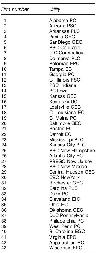
Our dataset is an updated and rened version of the panel of utilities originally analyzed by Nelson (1984). The primary sources for Nelson’s sample are the Federal Power Commis-sion’s Statistics of Privately Owned Electric Utilities in the U.S.,Steam Electric Plant Construction Cost and Annual Pro-duction Expenses, andPerformance Proles—Private Electric Utilities in the United States: 1963–70. Additional data were taken from Moody’s Public Utility Manual. The sample used here comprises 43 privately owned U.S. electric utilities oper-ating during the period 1961–1992, a span of 32 years. A list of the utilities, along with the rm number by which they are referenced in subsequent tables, is provided in Table 1. Because technologies for nuclear, hydroelectric, and internal combustion differ from that of fossil fuel-based steam gener-ation and because steam genergener-ation dominates total produc-tion by investor-owned utilities during the time period under investigation, we limit our analysis to fossil fuel–based steam electric generation.
Variable denitions are generally consistent with those in Nelson (1984). The inputs are fuel4E5, labor4L5, and capital
4K5and input quantities are measured as ratios of input expen-diture to price. The price of fuel is the dollar cost per mil-lion BTUs, computed as a consumption-weighted average for
Table 1. Utilities in the Sample
Firm number Utility
all fossil fuels. The wage rate is the sum of salaries and wages charged to electric operation and maintenance, divided by the sum of the number of full-time employees and one-half the number of part-time employees. The price of capital is computed using the yield of the rm’s latest issue of long-term debt adjusted according to the Christensen and Jorgenson (1970) cost of capital formula. In contrast to Nelson, we dis-tinguish between residential4R5and industrial-commercial4I5
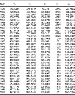
output. The output observations compiled by Daniel McFad-den and Thomas Cowing were updated using theStatistics of Privately Owned Electric Utilities in the U.S. The annual aver-ages for the quantities of all inputs and outputs, after division by their respective means, are presented in Table 2.
4.2 Speci’cation and Estimation of the Empirical Distance Function
Now we turn to the estimation of the TL distance func-tion in (22). Given the length of our panel, we rst consid-ered the possibility that the output and input variables in our sample might be nonstationary. We performed an augmented
Table 2. Average Quantities of Outputs and Inputs by Year
Year yR yIC xK xL xE
1961 168.3823 40709200 6604291 00800 6107289
1962 176.9538 43301858 10306655 00785 6405636
1963 192.4265 47002944 13206699 00785 6808821
1964 208.7739 51605051 15600270 00792 7504871
1965 222.0184 54908885 17302740 00812 8003374
1966 248.3429 61400524 15202298 00843 8909214
1967 259.7681 62303947 16300418 00877 9202113
1968 297.0779 69406430 17001343 00913 10302988
1969 321.9176 72909196 13801555 00927 11004089
1970 352.7994 76509681 21005131 00974 11706560
1971 364.9640 78700756 25607278 00973 12009622
1972 388.1944 84605498 45201978 01010 12801626
1973 408.7420 87908161 18903871 01081 13005623
1974 392.4335 84002874 29502266 01048 12701866
1975 398.5014 79505684 28503698 01028 15601618
1976 427.0868 88008098 27501169 01108 13503552
1977 447.0208 90704736 25006702 01156 14005621
1978 434.6622 87107672 25001362 01183 13701150
1979 446.3071 92106573 26108274 01251 14709652
1980 462.9539 90504313 27504478 01323 14401112
1981 457.4557 92908088 20003480 01353 14804255
1982 455.8784 88800466 18800279 01420 14004015
1983 446.5818 87804650 15700006 01436 14000112
1984 460.7704 93603479 15002297 01554 14709086
1985 458.9307 93906125 19806923 01459 15102314
1986 459.5176 91401424 17902839 01492 15408047
1987 480.7169 94704273 17300354 01473 14803831
1988 494.8696 98502379 23603905 01478 15601808
1989 514.6928 1104101288 29303866 01498 16200045
1990 487.7146 1100101416 20809623 01415 15600303
1991 487.3194 96506705 19907213 01347 15405238
1992 477.3123 97901402 18502413 01311 15207555
Dickey–Fuller (ADF) (Dickey and Fuller 1979) test for each of the 43 input and output series. Our test regressions included a constant, a linear and quadratic trend, and up to 10 aug-menting lags to account for dependence in the test regression errors. In general, we fail to reject the unit root null; on aver-age, for a given series, only 10% of the test statistics were signicant. However, the estimated value of the coefcient for the lagged dependent variable typically was not very close to 1. The average of this estimate for each output and input series, with zero augmenting lags for each input and output (so that the value of the coefcient under test would be as large as possible), ranged from .08 to .45.
With such sharp departures of these estimates from 1 and the well-known low-power of ADF tests, we prefer to take a Bayesian approach. Following Sims (1988) and Sims and Uhlig (1991), we treat the true value of the autoregressive parameter as a random variable centered at its estimated value. On average for each variable, at the .05 level with a one-tailed
ttest, we reject the null hypothesis that a root of 1 is included in the true value’s distribution 73% of the time. On this basis, we proceeded with estimation under the assumption that our output and input variables are stationary.
We next addressed the identication issue discussed in Section 3.4. We experimented with a variety of instrument sets, using Hansen’sJ test to determine the level of empirical support for the underlying moment conditions. For each case, we also calculated average annual PC, TC, and EC to gauge the sensitivity of these quantities to the choice of instruments. Table 3 reports the results from four different cases, which
Table 3. Sensitivity of Results to the Choice of Instruments
Instrument
set chi-squared df pvalue PC TC EC
1 52055 33 0017 0000470 0003910 ƒ0003440
2 39049 37 0359 0004647 0004582 0000064
3 38079 37 0389 0004673 0003570 0001103
4 104093 130 0948 0005635 0010917 ƒ0005282 NOTE: Each instrument set contains the linearly independent elements in A D [df1dt1dft1dft21d
ft3], wheretis a trend. The four cases are distinguished as follows:
(1)Aand[lnym1(lnym)21lnymlnyk]
(2)Aand[lnxn1(lnxn)21lnxnlnxl]
(3)Aand[lnpn1(lnpn)21lnpnlnpl]
(4) (3) and lnpndt, which includes each time realization of the input prices as a separate instrument in the spirit of Amemiya and MaCurdy (1986).
highlight the effects of including output or input quantities versus input prices in the instrument set. The precise distinc-tion between each case is provided in the notes to the table. The values of the test statistic, which are reported in the “chi-squared” column, soundly reject the use of output quantities (case 1), while giving support for the inclusion of input quan-tities or input prices (cases 2–4). Thep value associated with case 1 is only .017, but it exceeds .35 in the other three cases. Case 1 also yields an estimated annual PC rate that is an order of magnitude smaller than that produced by any of the other instrument sets. Although thep values are roughly the same for cases 2 and 3, we nd it more appealing on theoret-ical grounds to base estimation on the assumption that input prices are exogenous to electric utilities. Case 4 builds on this view by adding each time realization of the input prices as a separate instrument, in the spirit of Amemiya and MaCurdy (1986). With these additional instruments, the p value rises to .948, indicating strong support for this case. The estimated annual rate of PC is similar to that in cases 2 and 3, but the decomposition gives a much greater role to TC. Nevertheless, all three cases produce the same general temporal patterns in PC, TC, and EC, with the case 4 PC and TC (EC) series exhibiting slightly less (more) volatility than the other two cases. See the TL plots in Figures 1–3 in Section 4.3, where TL2–TL4 correspond to cases 2–4.
Given the results of J tests, and the increased precision afforded by the expanded instrument set in case 4, we base our nal estimation of (22) on these moment conditions. Over-all, this instrument set is generally highly correlated with the regressors, with theR2’s from the implied reduced forms rang-ing from .80 to .97. In estimation, we allow for heteroscedas-ticity and autocorrelation of unknown form, using the Newey and West (1987) covariance matrix estimator with 10 lags. The lag length was determined through an earlier Box–Jenkins analysis of the residual autocorrelations.
Two additional issues remain. The rst issue concerns the specication of technical change and technical inefciency. The empirical model described by (22) allows for the possibil-ity that temporal shifts in the distance function may be output and input augmenting. Because the model withƒmtDƒntD0,
8m1 n, and t failed to converge from numerous starting val-ues (regardless of the choice of instruments), we conclude that a specication of neutral technical change is appropriate for our utility data. Exploiting the model for technical inef-ciency given in (24) requires a value forQ. A likelihood ratio
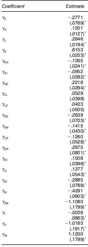
Table 4. Estimates of the Main
NOTE: Asymptotic standard errors are in parenthe-ses. An asterisk denotes signi’cance at the .05 level using a two-tailed test.
test, equal to the difference in the Hansen J statistic for the restricted and unrestricted models, rejects at the .05 level the null hypothesis that ‚fQD0, f D11 : : : 1 F, for QD2, but fails to reject at the .10 level forQD3. Likelihood ratio tests do not support adding higher-order trends, even if their coef-cients are restricted to be equal across rms. For this reason, we adopt a quadratic specication for theuft.
Given neutral technical change and Q D2, we have an empirical model with a total of 178 parameters. Perhaps not surprisingly, the overall t is good. TheR2 produced by esti-mating the normalized version of the model [described in (30)] exceeds .97 regardless of which input that we use as the regressand. Furthermore, estimates of the individual parame-ters are generally very precise. This is seen in the estimates of the main technology parameters (those associated with the outputs and inputs and their interactions) and their asymptotic standard errors reported in Table 4. It should be noted that almost the same level of precision is achieved in estimation of theƒt and‚fq; 80% of the former and 75% of the latter are signicant at the .10 level.
The second issue is whether (22) satises the curvature conditions for an input distance function, required for the duality between input prices and quantities. These conditions are that the distance function be monotonically increasing in inputs and monotonically decreasing in outputs, as well as quasi-concave in inputs. Our estimated model satises each of these properties at the mean of the relevant estimated princi-ple minors.
Finally, applying (21), we calculate the mean RTS for the entire sample to be 1.04 (with a range .8–1.3). A nding of this degree of increasing returns to scale is consistent with many previous empirical studies of U.S. electric utilities (e.g., Atkinson and Halvorsen 1984; Nelson 1984; Callan 1991). This feature of the data is not accommodated in DEA, which imposes an assumption of constant returns.
4.3 Estimation of Productivity Change
For each utility, we construct a Malmquist productivity index using DEA, which requires us to solve a series of lin-ear programming problems as outlined by FGNZ. In doing so, we follow the standard practice of maintaining CRS. We then decompose each rm-specic index of PC into EC and TC, following FGNZ.
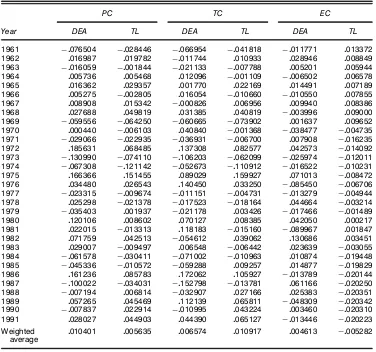
Following estimation of (22), we compute EC using (27), TC using (28), and PC using (13). Tables 5 and 6 report the industry weighted-average PC, TC, and EC by year and rm, as computed with DEA and estimated from our TL frontier distance function. The weights in each case are revenue shares. Consider rst the rates of change presented in Table 5. The last row of the table provides the average annual rate of PC, TC, and EC over the entire 32-year period and high-lights one of the main points of contrast between the DEA and TL results. Whereas DEA and TL estimation yield somewhat similar annual rates of PC, 1.04% versus .56%, they conict sharply on which source, TC or EC, is more important. From the TL estimates, we calculate average annual TC of 1.09% and EC of ƒ053%, which implies that TC is responsible for all of the productivity gain over the period. The DEA-based Malmquist indices lead to a more balanced decomposition, producing average annual TC of about .66% and EC of about and .46%. One explanation is that much of what DEA counts as EC, the stochastic distance function nets out as noise. In any event, the idea that TC is the primary force behind PC among electric utilities seems reasonable in light of regulation that has historically provided incentives for utilities to invest in capital, but has provided few competitive forces to spur improvements in technical efciency.
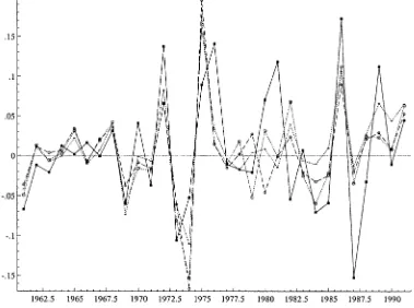
A second important distinction between the DEA and TL rates of change is the generally sharper year-to-year uctua-tions in the former. This is seen in the plots of the DEA and TL PC, TC, and EC series provided in Figures 1–3. Note in particular the contrast between DEA and TL4 PC series over the periods 1971–1973, 1979–1981, and 1985–1987, when the DEA (TL)-based PCs moved from ƒ3% to 19% to ƒ13% (ƒ2% to 7% to ƒ7%), ƒ4% to 12% to 2% (.2% to .9% to
ƒ1%), and ƒ5% to 16% to ƒ10% (ƒ1% to 9% to ƒ3%). Interestingly, both methodologies capture large swings in pro-ductivity from 1974 to 1976. The inuence of the OPEC oil
Table 5. Industry Weighted-Average Rates of Change by Year
PC TC EC
Year DEA TL DEA TL DEA TL
1961 ƒ0076504 ƒ0028446 ƒ0066954 ƒ0041818 ƒ0011771 0013372
1962 0016987 0019782 ƒ0011744 0010933 0028946 0008849
1963 ƒ0016059 ƒ0001844 ƒ0021133 ƒ0007788 0005201 0005944
1964 0005736 0005468 0012096 ƒ0001109 ƒ0006502 0006578
1965 0016362 0029357 0001770 0022169 0014491 0007189
1966 0005275 ƒ0002805 0016054 ƒ0010660 ƒ0010550 0007855
1967 0008908 0015342 ƒ0000826 0006956 0009940 0008386
1968 0027688 0049819 0031385 0040819 ƒ0003996 0009000
1969 ƒ0059556 ƒ0064250 ƒ0060665 ƒ0073902 0001637 0009652
1970 0000440 ƒ0006103 0040840 ƒ0001368 ƒ0038477 ƒ0004735
1971 ƒ0029066 ƒ0022935 ƒ0036931 ƒ0006700 0007908 ƒ0016235
1972 0185631 0068485 0137308 0082577 0042573 ƒ0014092
1973 ƒ0130990 ƒ0074110 ƒ0106203 ƒ0062099 ƒ0025974 ƒ0012011
1974 ƒ0067308 ƒ0121142 ƒ0052673 ƒ0110912 ƒ0016522 ƒ0010231
1975 0166366 0151455 0089029 0159927 0071013 ƒ0008472
1976 0034480 0026543 0140450 0033250 ƒ0085450 ƒ0006706
1977 ƒ0023315 ƒ0009674 ƒ0011151 ƒ0004731 ƒ0013279 ƒ0004944
1978 0025298 ƒ0021378 ƒ0017523 ƒ0018164 0044664 ƒ0003214
1979 ƒ0035403 0001937 ƒ0021178 0003426 ƒ0017466 ƒ0001489
1980 0120106 0008602 0070127 0008385 0042050 0000217
1981 0022015 ƒ0013313 0118183 ƒ0015160 ƒ0089967 0001847
1982 0071759 0042513 ƒ0054612 0039062 0130686 0003451
1983 0029007 ƒ0009497 0006548 ƒ0006442 0023639 ƒ0003055
1984 ƒ0061578 ƒ0030411 ƒ0071002 ƒ0010963 0010874 ƒ0019448
1985 ƒ0045336 ƒ0010572 ƒ0059288 0009257 0014877 ƒ0019829
1986 0161236 0085783 0172062 0105927 ƒ0013789 ƒ0020144
1987 ƒ0100022 ƒ0034031 ƒ0152798 ƒ0013781 0061166 ƒ0020250
1988 ƒ0007194 0006814 ƒ0032907 0027166 0025383 ƒ0020351
1989 0057265 0045469 0112139 0065811 ƒ0048309 ƒ0020342
1990 ƒ0007837 0022914 ƒ0010995 0043224 0003460 ƒ0020310
1991 0028027 0044903 0044390 0065127 ƒ0013446 ƒ0020223
Weighted 0010401 0005635 0006574 0010917 0004613 ƒ0005282
average
embargo is probably part of the explanation; other studies (e.g., Nelson and Wohar 1983) have observed the same kind of period-to-period changes. However, it is perhaps notewor-thy thatƒO75is not statistically signicant at any reasonable test size, with the implication being that the TL estimate of .15 for the PC rate in 1975 should not be taken seriously. In con-trast, DEA, which yields a PC rate of .16 in 1975, provides no statistical evidence with which to gauge the reliability of this result.
We regard annual shifts in productivity of these magni-tudes to be implausible. Such large uctuations in PC, which are paralleled in the DEA TC and EC series, are most likely due to the failure of DEA to account for noise. Another possible contributing factor is that the nonparametric DEA-constructed technology is not a very good approximation to the true technology. If so, the nonparametric “robustness” of DEA loses its appeal. This is essentially the conclusion of Gong and Sickles (1992), whose Monte Carlo evidence sug-gests that stochastic frontier estimation is preferable to DEA when a parametric functional form can be found that closely approximates the underlying technology.
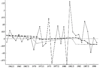
Although more volatile, the DEA-based average annual PC and TC series track those derived from the TL distance func-tion fairly closely. The correlafunc-tion coefcients between the two PC series is .82, and that between the two TC series is .62. The temporal patterns of the EC series are considerably less
similar. The combination of our stochastic frontier and para-metric specication for technical inefciency has smoothed out much of the extreme period-to-period swings in EC. As a result, the correlation coefcient between the EC series is only .02.
Because no previous study of U.S. electric utilities has examined the productivity of the 43 utilities in our sample over the 1961–1992 time period, we do not have a benchmark against which to compare the series plotted in Figures 1–3. More signicantly from our perspective, earlier studies typi-cally were not concerned with decomposing PC into TC and EC. In any event, a number of researchers (e.g., Nelson and Wohar 1983; Baltagi and Grifn 1988; Callan 1991) have ana-lyzed the productivity of U.S. electric utilities using some sub-set of the rms in Nelson’s (1984) datasub-set over time periods extending from the 1950s through the early 1980s, producing estimates of average annual TC in the range of .7 to 1.7.
Finally, we examine the average annual rates of change reported for each utility in Table 6. The DEA and TL models identify different rms as experiencing the largest and small-est productivity gains over the period. The DEA method indi-cates that PSEGC New Jersey (Cleveland EIC) has the fastest (slowest) rate of growth, with an average annual PC of 7.1% (ƒ045%), whereas the estimated TL nds that PC Iowa and Kansas GEC (Carolina PLC) have (has) the fastest (slowest) rate of growth, with an average annual PC of 1.9% (ƒ063%).
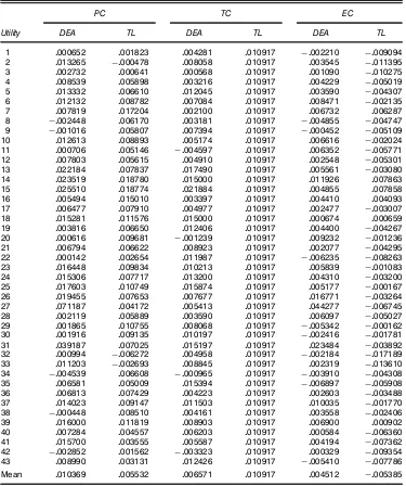
Table 6. Average Annual Rates of Change by Utility
PC TC EC
Utility DEA TL DEA TL DEA TL
1 0000652 0001823 0004281 0010917 ƒ0002210 ƒ0009094
2 0013265 ƒ0000478 0008058 0010917 0003545 ƒ0011395
3 0002732 0000641 0000568 0010917 0001090 ƒ0010275
4 0008539 0005898 0003216 0010917 0004229 ƒ0005019
5 0013332 0006610 0012045 0010917 0003590 ƒ0004307
6 0012132 0008782 0007084 0010917 0008471 ƒ0002135
7 0007819 0017204 0002100 0010917 0006732 0006287
8 ƒ0002448 0006170 0003181 0010917 ƒ0004855 ƒ0004747
9 ƒ0001016 0005807 0007394 0010917 ƒ0000452 ƒ0005109
10 0012613 0008893 0005174 0010917 0006616 ƒ0002024
11 0000706 0005146 ƒ0004597 0010917 0006352 ƒ0005771
12 0007803 0005615 0004910 0010917 0002548 ƒ0005301
13 0022184 0007837 0017490 0010917 0005561 ƒ0003080
14 0023519 0018780 0015000 0010917 0011926 0007863
15 0025510 0018774 0021884 0010917 0004855 0007858
16 0005494 0015010 0003397 0010917 0004410 0004093
17 0006477 0007910 0004977 0010917 0002477 ƒ0003007
18 0015281 0011576 0015000 0010917 0000674 0000659
19 0003816 0006650 0012406 0010917 0004400 ƒ0004267
20 0000616 0009681 ƒ0001239 0010917 0009232 ƒ0001236
21 0006794 0006622 0008923 0010917 0002077 ƒ0004295
22 0000142 0002654 0011987 0010917 ƒ0006235 ƒ0008263
23 0016448 0009834 0010213 0010917 0005839 ƒ0001083
24 0015306 0007717 0013200 0010917 0004310 ƒ0003200
25 0017603 0010749 0015874 0010917 0005177 ƒ0000167
26 0019455 0007653 0007677 0010917 0016771 ƒ0003264
27 0071187 0004172 0005413 0010917 0044277 ƒ0006745
28 0002119 0005889 0003590 0010917 0006097 ƒ0005027
29 0001865 0010755 0008068 0010917 ƒ0005342 ƒ0000162
30 0001916 0009135 0010197 0010917 ƒ0002416 ƒ0001781
31 0039187 0007025 0015197 0010917 0023484 ƒ0003892
32 0000994 ƒ0006272 0004958 0010917 ƒ0002184 ƒ0017189
33 0011203 ƒ0002693 0008845 0010917 0002319 ƒ0013610
34 ƒ0004539 0006608 ƒ0000965 0010917 ƒ0003910 ƒ0004308
35 0006581 0005009 0015394 0010917 ƒ0006897 ƒ0005908
36 0006813 0007429 0004223 0010917 0002603 ƒ0003488
37 0014023 0009147 0011503 0010917 0010035 ƒ0001770
38 ƒ0000448 0008510 0004161 0010917 0003558 ƒ0002406
39 0016000 0011819 0008903 0010917 0006900 0000902
40 0007284 0004557 0006203 0010917 0000584 ƒ0006360
41 0015700 0003555 0005587 0010917 0004194 ƒ0007362
42 ƒ0002852 0001562 ƒ0003323 0010917 0000329 ƒ0009354
43 0008990 0003131 0012426 0010917 ƒ0005410 ƒ0007786
Mean 0010369 0005532 0006571 0010917 0004512 ƒ0005385
Overall, the rank correlation between the two sets of average annual rates of PC is .34.
5. SUMMARY AND CONCLUSIONS
Following FGNZ, measuring PC with Malmquist indices has become common practice, because these are easily com-puted using the nonparametric programming techniques of DEA and can be readily decomposed into TC and EC. How-ever, this approach has two major problems. First, a CRS fron-tier technology is used to compute PC. This is overly restric-tive, because the Malmquist index is valid for any degree of returns to scale. Second, DEA is deterministic, so statis-tical inference is precluded without a change in the initial assumption that DEA scores are nonstochastic. In addition, because DEA is deterministic, all departures from the DEA frontier are treated as inefciency, so that noise is included in the measure of efciency change.
We propose an alternative econometric approach that com-bines and extends the best elements of each approach. First, we estimate a exible, parametric stochastic distance function that accounts for technical inefciency. The exible nature of our distance frontier allows us to compute PC without arbi-trarily restricting returns to scale. The stochastic nature of our frontier allows us to distinguish technical inefciency from random variations in the frontier and to conduct specica-tion tests along with tests of the usual parametric hypothe-ses. Within this framework, we obtain a decomposition for PC analogous to that of FGNZ. To our knowledge, this result has not been established and implemented for a parametric stochastic distance frontier. Finally, we formulate a GMM esti-mation strategy for the frontier distance function that does not restrict either outputs or inputs to be exogenous.
Using a newly updated panel of U.S. electric utilities, we contrast the DEA and econometric approaches. With DEA, we
Figure 1. PC for DEA and TL (ÿ ÿDEAyear;- - -TL2year;&: : :&TL3year;: : : TL4year).
nd an average annual rate of PC of 1.04%, versus .56% as derived from our estimated TL. More striking is the difference between the two methodologies in the relative importance that each assigns to TC and EC. The estimated TL attributes all of
Figure 2. TC for DEA and TL (ÿ ÿDEAyear;- - -TL2year;&: : :&TL3year;: : : TL4year).
the average productivity gain to TC, whereas DEA yields more balance in the measured sources of PC. In addition, the DEA series exhibits much greater volatility over time. We argue that these disagreements are most likely due to the failure of DEA
Figure 3. EC for DEA and TL (ÿ ÿDEAyear;- - - TL2year;&: : :&TL3year;: : : TL4year).
to account for noise, with the DEA’s assumption of CRS also playing a role.
ACKNOWLEDGMENTS
We are very grateful to the editor and an associate editor for their very careful reviews of earlier drafts of this article. We also thank Rolf F¨are for his helpful comments, and Professor Nelson for making his data available to us.
[Received June 1998. Revised September 2001.]
REFERENCES
Amemiya, T., and MaCurdy, T. E. (1986), “Instrumental-Variable Estimation of an Error-Components Model,”Econometrica, 54, 869–880.
Atkinson, S. E., and Halvorsen, R. (1984), “Parametric Efciency Tests, Economies of Scale, and Input Demand in U.S. Electric Power Genera-tion,”International Economic Review, 25, 647–662.
Baltagi, B. H., and Grifn, J. M. (1988), “A General Index of Technical Change,”Journal of Political Economy, 96, 20–41.
Callan, S. J. (1991), “The Sensitivity of Productivity Growth Measures to Alternative Structural and Behavioral Assumptions: An Application to Electric Utilities 1951–1984,”Journal of Business and Economic Statistics, 9, 207–213.
Caves, D. W., Christensen, L. W., and Diewert, W. E. (1982), “The Economic Theory of Index Numbers and the Measurement of Input, Output, and Pro-ductivity,”Econometrica, 50, 1393–1414.
Christensen, L. R., Caves, D. W., and Swanson, J. A. (1981), “Productiv-ity Growth, Scale Economies, and Capac“Productiv-ity Utilization in U.S. Railroads, 1955–74,”American Economic Review, 71, 994–1002.
Christensen, L. R., and Jorgenson, D. W. (1970), “U.S. Real Product and Real Factor Input, 1928–1967,”Review of Income and Wealth, 16, 19–50. Coelli, T., and Perelman, S. (1996), “Efciency Measurement,
Multiple-Output Technologies and Distance Functions: with Application to European Railways,” CREPP working paper 96/05, University of Liège, Belgium. Cornwell, C., Schmidt, P., and Sickles, R.C. (1990), “Production Frontiers
With Time Series Variation in Efciency Levels,”Journal of Econometrics, 46, 185–200.
Dickey, D. A., and Fuller, W.A. (1979) “Distribution of the Estimators for Autoregressive Time Series With a Unit Root,”Journal of the American Statistical Association, 74, 427–431.
F¨are, R., Grosskopf, S., Norris, M., and Zhang, Z. (1994), “Productivity Growth, Technical Progress, and Efciency Change in Industrial Coun-tries,”American Economic Review, 84, 66–83.
F¨are, R., and Primont, D. (1996), “The Opportunity Cost of Duality,”Journal of Productivity Analysis, 7, 213–224.
Gong, B., and Sickles, R. (1992), “Finite Sample Evidence on the Perfor-mance of Stochastic Frontiers and Data Envelopment Analysis Using Panel Data,”Journal of Econometrics, 51, 259–284.
Good, D., and Sickles, R. (1997), “Specication of Distance Functions Using Semi- and Nonparametric Methods With an Application to Eastern and Western European Air Carriers,” working paper, Rice University. Grosskopf, S., Hayes, K., Taylor, L., and Weber, W. (1997), “Budget
Con-strained Frontier Measures of Fiscal Equality and Efciency in Schooling,”
Review of Economics and Statistics, 79, 116–124.
Hansen, L. P. (1982), “Large Sample Properties of Generalized Method of Moments Estimation,”Econometrica, 50, 1029–1054.
Moody’s Investors Service (various years),Moody’s Public Utility Manual, New York: author.
Nelson, R. A. (1984), “Regulation, Capital Vintage, and Technical Change in the Electric Utility Industry,”Review of Economics and Statistics, 66, 59–69.
Nelson, R. A., and Wohar, M. (1983), “Regulation, Scale Economies, and Pro-ductivity in Steam-Electric Generation,” International Economic Review, 24, 57–59.
Newey, W. K., and West, K. D. (1987) “A Simple, Positive Semi-Denite, Het-eroskedasticity and Autocorrelation Consistent Covariance Matrix,” Econo-metrica, 55, 703–706.
Ray, S. C., and Desli, E. (1997), “Productivity Growth, Technical Progress, and Efciency Change in Industrial Countries: Comment,”American Eco-nomic Review, 87, 1033–1039.
Sims, C. (1988), “Bayesian Skepticism on Unit Root Econometrics,”Journal of Economic Dynamics and Control, 12, 463–474.
Sims, C., and Uhlig, H. (1991), “Understanding Unit Rooters: A Helicopter Tour,”Econometrica, 59, 1591–1599.
U.S. Federal Power Commission (annually),Statistics of Privately Owned Electric Utilities in the U.S.—Classes A and B, Washington, DC: U.S. Government Printing Ofce.
(annually),Steam Electric Plant Construction Cost and Annual Pro-duction Expenses, Washington, DC: U.S. Government Printing Ofce.
(annually), Performance Proles—Private Electric Utilities in the United States: 1963–70, Washington, DC: U.S. Government Printing Ofce.