El e c t ro n ic
Jo ur
n a l o
f P
r o
b a b il i t y
Vol. 15 (2010), Paper no. 24, pages 723–740. Journal URL
http://www.math.washington.edu/~ejpecp/
IDLA on the Supercritical Percolation Cluster
Eric Shellef
The Weizmann Institute of Science 76100 Rehovot
Israel [email protected]
Abstract
We consider the internal diffusion limited aggregation (IDLA) process on the infinite cluster in supercritical Bernoulli bond percolation onZd. It is shown that the process on the cluster
behaves like it does on the Euclidean lattice, in that the aggregate covers all the vertices in a Euclidean ball around the origin, such that the ratio of vertices in this ball to the total number of particles sent out approaches one almost surely.
Key words:.
AMS 2000 Subject Classification:Primary 60K35.
1
Introduction
1.1
Background and discussion
Given a graph, IDLA defines a random aggregation process, starting with a single vertex and growing by a vertex in each time step. To begin the process, we specialize a vertexvto be the initial aggregate on the graph. In each time step, we send out one random walk from v. Once this walk exits the aggregate, it stops, and the new vertex is added to the aggregate. LetI(n)be the aggregate in step
n, thusI(1) ={v}and|I(n)|=n.
This process is a special case of a model Diaconis and Fulton introduced in[DF91]. In the setting where the graph is thed-dimensional lattice, Lawler, Bramson and Griffeath in[LBG92]used Green function estimates to prove the process has a Euclidean ball limiting shape. Let Br be all vertices in Zd of Euclidean distance less than r from the origin. The main theorem in [LBG92] implies that for anyε > 0, I(BR
)⊃ B(1−ε)R for all sufficiently largeR with probability one. Seeking to generalize this result to other graphs, we note that convergence of a random walk on the lattice to isotropic Brownian motion plays an important role in convergence of IDLA on the lattice to an isotropic limiting shape.
However, this property by itself is in general not enough for IDLA to have such an inner bound, as the following example shows. Consider the three dimensional Euclidean lattice, and choose a vertex
v at distance R from the origin. Let r = R0.9 and let Br(v) be the set of vertices of distance less than r from v. Remove all edges but one from the boundary of Br(v), and denote by v′ the only vertex inBr(v)with a neighbor outside ofBr(v). Let us look atI(B2R
). A rough calculation gives that the average number of visits tov′is of orderR−1B2R
. Since at least Br(v)
=R2.7 visits tov′ are needed to fillBr(v), we don’t expect the ball to be full after an order ofR3 particles have been sent out. Repeating this edge removal procedure for balls of radius R0.9n at distanceRn from the origin whereRn=2nR, will ensure that there is never a Euclidean inner bound. However, a random walk from the origin on this graph will converge to Brownian motion because our disruptions are sublinear. We will not give full proofs of these facts, but hope they convince the reader that to get an inner bound some kind of local regularity property is needed.
The main theorem of this paper states that IDLA on the supercritical cluster in the lattice has a Euclidean ball as an inner bound. The two main tools that are used to show this are a quenched invariance principle[BB07]which gives us convergence in distribution to Brownian Motion from a fixed point, and a Harnack inequality from[Bar04], which give us oscillation bounds on harmonic functions in all small balls close to the origin. The latter allows us to establish the local regularity missing from the above example.
1.2
Assumptions and statement
Consider supercritical bond percolation inZd with the origin conditioned to be in the infinite cluster.
Let the graph Γ(V,E) be the natural embedding in Rd of the infinite cluster, i.e. V ⊂ Rd. Fixing
this embedding for Γ, we get two separate (but comparable, see [AP96]) distances. We denote by x−y
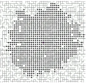
Figure 1.1:IDLA of 1000 particles from marked vertex on the percolation cluster withp=0.7.
following: br(x) ={y∈Rd |d(x,y)<r}. Letdr(x)be a box of sider with centerx, and as above,
letDr(x)be the vertices in this box.
By existing work, which we will reference later, we know that with probability one, the graph of the supercritical cluster,Γ, in its naturalRd embedding, satisfies the following assumptions:
1. A random walk onΓconverges weakly in distribution to a Brownian Motion as defined in 1.4.
2. Convergence to vertex densityaG>0 as defined in 1.5.
3. A uniform upper bound on exit time from a ball as defined in 1.6.
4. A Harnack inequality as defined in 1.7.
We denote byXt a discrete “blind” random walk onΓdefined as follows. Forx∈Γandt∈N∪ {0},
P Xt+1= y|Xt=x
=1/2d if y is a neighbor ofx inΓ, andP Xt+1=x|Xt=x
=1−degx/2d. We prefer this walk since its Green functions are symmetric, a fact which will be useful later on. For non-integert we setXt=X⌊t⌋.
Note that assumption 4 does not imply 3, see[Del02]for a counterexample.
Using only above assumptions and thatV ⊂Zd (which serves mostly to simplify notation and could
be replaced by weaker conditions), we show the IDLA process starting at0 will have a Euclidean ball inner bound as stated in the following theorem:
LetI(n)denote the random IDLA aggregate ofnparticles starting at0.
Theorem 1.1. Almost surely, for anyε >0, we have that for all large enough R, B(1−ε)R⊂ I( BR
)
1.3
Outline
In the remainder of this section we state our assumptions precisely, and explain why these assump-tions are valid almost surely for the infinite cluster in supercritical percolation.
Then, to prove IDLA inner bound, we need to show that for each vertexv ∈V the Green function from0and expected exit time from a ball around0of a random walk starting atv, behave similarly to those functions of a Brownian motion. The exact statement needed appears in Lemma 3.1. The invariance principle gives us integral convergence of these functions to the right value, but to improve them to pointwise statements, we must show that they are locally regular. We use the Harnack inequality from[Bar04]to prove they are Hölder continuous. This is a similar scheme to improving a CLT to an LCLT, as was done in[BH09]using a different method than ours.
In section 2, we start by proving a lemma comparing expected exit time from a set to the Green function of a point in the set. Then, we show how our Harnack assumption leads to an oscillation inequality which we use to show regularity of the Green function and expected exit time of the walk in a ball when we are far from the boundary and the center. Next, in section 3, we use our assumption of an invariance principle to show that in small balls the integral of these functions approaches a tractable limit that can be calculated by knowledge of Brownian motion. Finally, in section 4, we utilize these estimates to prove theorem 1.1.
Remark1.2. Since the paper makes use of results based on ergodic theory, there is no rate estimate for the convergence in theorem 1.1. Also, on the Euclidean lattice there is an almost sure outer bound with sublinear fluctuations from the sphere. Another interesting question that is not treated here, is whether a similar outer bound holds in our setting.
1.4
Weak convergence to Brownian Motion
In this and the next three subsections, we give a precise formulation of each of our assumptions from above, and argue that they hold a.s. onΓ, the supercritical cluster.
Let CTd = C([0,T] → Rd), i.e. the continuous functions from the closed interval [0,T] to d
-dimensional Euclidean space. ForR∈N, let
wR(t) = 1
R
X⌊tR2⌋+ (tR2− ⌊tR2⌋)(X⌊tR2⌋+1−X⌊tR2⌋)
.
Thus wR(t) is a scaled linear interpolation of Xt (defined in 1.2) with its restriction to [0,T]an element ofCTd.
We say that assumption 1 holds if for any T >0, the law ofwR(t) onCTd converges weakly in the supremum topology to the law of a (not necessarily standard) Brownian Motion(Bt: 0≤t≤T).
Lemma 1.3. Assumption 1 holds forΓwith probability one.
Proof. This is Theorem 1.1 in[BB07]. Another paper with a similar invariance principle is[MP05].
1.5
Convergence to positive density
Assumption 2 holds if there exists a positiveaGsuch that for anyδ,γ >0 and all sufficiently largeR we have that for all x∈bRand allδR≤r≤R
Lemma 1.4. Assumption 2 holds forΓwith probability one.
Proof. Letθ(p)be the probability for0to be in the infinite cluster.θ(p)is positive in the supercrit-ical regime. From Theorem 3 in[DS88]ford=2 and from (2) on p. 15 of[Gan89]ford>2, we
x. Theorem 2 in [DS88] proves the easier density upper bound for d = 2, which under trivial modifications gives that for alld
Pn−dDn(x)
>(1+ρ)θ(p)
<exp(−cn).
The above, together with Borel Cantelli gives that if we chooseγ > 0, x ∈b1, then for all large enoughR enough so that the number of boxes that intersect both DandDR\Dis negligible compared to the number that intersectD. Proving for balls is similar.
1.6
Uniform Bound on Exit time from ball
Denote byτr(x)the first time the walk leavesBr(x), and writeτr forτr(0).
The assumption holds forΓwith probability one as a direct consequence of the following lemma, proved below.
Lemma 1.5. With probability one, there is an L such that for all δ > 0and all large enough R, if x ∈BRand r> δR then
Proof. Since we prove for allRoutside a bounded interval, it suffices to prove the above forr=δR
with fixedδ >0. To prove this holds a.s. for supercritical percolation clusters, we use a heat kernel upper bound given in Theorem 1 of Barlow’s paper[Bar04]. The proof in[Bar04]is for continuous walks with a mean time of one between jumps. However, it can be transferred to our discrete walk using Theorem 2.1 of[BB07]. We state an implication of what was proved.
With probability one there exists a function fromV toN,Tx <∞
Barlow’s result actually states that almost surelyTx grows slower than a logarithmic function ofkxk
and gives stronger Gaussian bounds for the heat kernel from below and above.
Using the heat kernel upper bound (1.3), the convergence to zero of Tx
kxk, and the upper bound on
We rewrite the left hand side of (1.4) and use the Markov property with the exit time assumption.
Since ExτR/R2
is bounded by cE for all R, we have by the Markov inequality that P(τR/R2 >
T)≤cE/T which converges to zero as T goes to∞uniformly inRfor all x∈BR.
1.7
Harnack inequality
A function h : Γ → R is harmonic on x ∈ Γ if h(x) = |N(x)|−1P
y∈N(x)h(y) where N(x) =
y ∈Γ:dΓ(x,y) =1 are the neighbors of x. We say his harmonic on Z ⊂ Γ if it harmonic on every vertexv∈Z.
Assumption 4 holds if there is a 1<cH<∞such that for allδ >0 we have that for all large enough
R, if x ∈BR, r> δRandhis a function that is non-negative and harmonic onB2r(x)then
sup Br(x)
h≤cH inf Br(x)
h. (1.5)
In order to simplify the paper, the inequality above is formulated for Euclidean distance rather than graph distance. We show that since the distances are almost surely comparable onΓ, this is the same. We start by proving the assumption holds for graph distance, using Lemma 2.19 and Theorem 5.11 of[Bar04]. We write BΓr =
x∈Γ:dΓ(0,x)≤r) . The lemma, using appropriate parameters and Borel Cantelli, tells us that for all large enough R, BRΓlogR arevery good balls. Specifically, all balls contained inBRΓlogRof graph radius larger thanR1/4(d+2)have a positive volume density and satisfy a weak Poincaré inequality as explained in (1.15) and (1.16) of the same. Theorem 5.11 then tells us that for very good ball of graph radiusRlogR, all x ∈BΓ
(RlogR)/3 satisfy that for any functionh
non-negative harmonic onBRΓ(x)
sup BΓR/2(x)
h≤ˆcH inf BΓ
R/2(x)
h (1.6)
where ˆcH(d,p) >0 is a constant dependent only on dimension and percolation probability. Since all but a finite number of balls of graph radius RlogR are very good and R is o(RlogR) we have assumption 4 for graph distance.
Next, we transfer this to the Euclidean balls formulation of (1.5). By Theorem 1.1 of[AP96], we have that for somek>0,ρ(d,p)>0 andM <∞,
P
dΓ(x,y)> ρm
x,y ∈Γ, x−y
=m>M
<exp(−km).
Let A(x,y) be the event
dΓ(x,y)> ρm . Union bounding the probability for A(x,y) over every pair of points inBRof Euclidean distance greater thanclogRfor some large c(k), we upper bound the probability of any such event occuring by
CRd
∞ X
m=clogR
md−1exp(−km)<C′Rd logRd−1
R−2d,
which is summable ford>1. Hence by Borel Cantelli, almost surely for all large enoughR, we have that for any x,y ∈BRwithx− y
>clogR, dΓ(x,y)< ρ x− y
. Since logR iso(R), this implies that for anyδ >0 and all large enoughR, for anyx ∈BR,
Note thatBΓr(x)⊂Br(x)always becauseΓis embedded inZd. Hence, given a function that is
non-negative harmonic onB2r(x)it is also such onBΓ2r(x). For large enough R, we use (1.6) and (1.7) to get (1.5) forBρ−1r(x)with constantˆcH. A routine chaining argument (see e.g. (3.5) in[Del02])
transfers this toBr(x)as required with new constantcH.
2
Pointwise bounds on Green function and expected exit time
In this section, we show the assumptions of a uniform bound on exit time from a ball along with the Harnack inequality give us pointwise bounds of the Green function and expected exit time of a random walk.
As a convention, we use plainc and C to denote positive constants that do not retain their values from one expression to another, as opposed to subscripted constants ci, that do. In general, these constants are graph dependent, and in the context of percolation, can be seen as random functions of the percolation configuration. However, we view the graph as being fixed and satisfying the assumptions stated in subsection 1.2.
We start with a general lemma on the relation between expected exit time from a set and the expected number of visits to a fixed point in the set.
Let Z ⊂ Γ and let τZ be the first hitting time of Z for Xt. For x ∈ Γ we set GZ(x) =
Ex hPτ
Z
t=01{Xt=x}
i
, the expected number of visits to x of a walk starting at x beforeτZ.
Lemma 2.1. There is a k=k(d)>0such that for any x∈Γand Z⊂Γwhere N(x)∩Z=;
Ex τZ
>kG2Z/logGZ. (2.1)
Proof. Recall from 1.2 thatXt has a positive staying probability at certain vertices. Since we apply electrical network interpretation to estimate hitting probabilities, we prove the above for Yt, the usual discrete simple random walk, with 0 probability to stay at a vertex. This implies (2.1) forXt
as well, since the expected exit time cannot decrease, and the Green functions forXt can only grow by a 2d factor since the escape probabilites forXt andYtare at most a 2d factor apart.
Fixx ∈Γ, setT0=0, and define for eachi∈Nthe r.v.’s
Ti=inft>Ti−1:Yt= x .
Let i∗ =inf
i:Ti=∞ . For 1 ≤ i≤ i∗ let ρi = Ti−Ti−1. We show there are positive constants k1,k2 dependent only ond such that
Pρ1≥k1r2/logr
≥ k2
r . (2.2)
For some r > 1, let ∂BΓr(x) =
v∈Γ:dΓ(v,x) =r . By electrical network interpretation (see
e.g. [DS84]), the probability for a walk beginning at x to hit ∂BΓr(x) before returning to x is
(2d)−1C
Next, let y ∈∂BΓr(x). By the Carne-Varopoulos upper bound (see[Var85]),
P
Yt=x|Y0= y
≤4d1/2exp
−r 2
2t
and thus, for somek1(d),k2(d)>0 and allr>1, the probability that a walk starting at y∈∂BΓr(x)
does not hit x in the next⌊k1r2/logr⌋steps, by union bound, is greater thank2. Together with our
lower bound on the probability that we arrive at such a y ∈∂BΓr(x), we get (2.2). Next, let g=inf
i:Ti> τZ be the number of visits ofYt tox before hittingZ, includingt=0 . g
is a geometric random variable with meanG=GZ. Letα= 12ln(4/3)and note that since there is a constant in (2.1) andτZ ≥1, we can assumeG>2. Thus
P
g≥αG ≥
1−G−1αG
≥ 1−G−12α(G−1) ≥ e−2α=3/4
We further assumeG > 2α∨16k
2 so thatαG−1> αG/2 andG
k2
16 >1. Let Abe the event that there
is an 1≤i≤(αG−1)∧i∗ such thatρi >k1
k
2
16G
2
/logk2
16G
Note thati∗≤αG−1 impliesA. Thus by (2.2) and the independence of consecutive excursions fromx,
P[Ac]≤
1−16
G
αG/2
≤e−8α
which is smaller than 1/4. Thus
P
g≥αG ,A
≥ 1
2.
This implies the lemma sinceτZ >Pig=−11ρi, and fork=k1k22/256,
Pg−1
i=1 ρi >kG2/logG.
Next, we state the fact that a Harnack inequality implies an oscillation inequality. For a set of vertices
U and a functionu, let
oscU(u) =maxU(u)−minU(u).
Proposition 2.2. Let x ∈Γand assume that for some r >0we have that any function h that is non-negative and harmonic on B2r(x)satisfies(1.5)on Br(x). Then for any h that is harmonic on B2r(x), we have
oscB
r(x)h≤
cH−1
cH+1oscB2r(x)h. (2.3)
Proof. We quote a proof from chapter 9 of[Tel06].
Set v = h−minB
2r(x)h. Since v is non-negative and harmonic on B2r(x), the Harnack inequality
(1.5) is satisfied here, so we have
max Br(x)
v≤cHmin Br(x)
whence
Summing up these two inequalities, we obtain
oscBr(x)h≤
Iterating this on the Harnack assumption 4 we get
Corollary 2.3. For anyα >0there is an M(α)such that for anyη >0and for all R>Rη, if x ∈BR,
r≥ηR and h is a harmonic function on BM(α)r(x)then
oscBr(x)h≤αoscBM r(x)h.
We use this to show regularity of the green function and for expected exit time.
Lemma 2.4. There is a cG(ε)such that for all large enough R, and any x∈B(1−ε)R\BεR
Lemma 2.6. For any β >0, there is a δ > 0such that for all large enough R, any x,y ∈ B(1−ε)R βR2/2. Applying the triangle inequality finishes the proof.
3
Domination of Green function
LetΩ = ΓN∪{0} and letPB(·)denote a probability measure on paths inΩstarting at0that makeX t a “blind” simple random walk as defined in subsection 1.2. PB is pushed forward to a measure on
Cd
T bywR(t) as defined in subsection 1.4. To contrast, we call P(·)the Wiener measure on curves corresponding to the Brownian motionB(t)which is the weak limit of wR(t). Thus, for fixed T,
CTd is the probability space on which PB wR(t)
converges to P in distribution. Write EB[·]and
E[·]for the corresponding expectations.
3.1
Integral Convergence of expected exit time
Since we assume control of convergence to Brownian Motion only from 0, we must describe the expected exit time from an arbitrary point in the unit ball as a function of Brownian motion that starts at0. We do this by conditioning the Brownian motion to hit a small box containing that point and measuring the additional time needed to exit the unit ball.
We denote the first hitting time of a set Z by τZ. This hitting times may refer to the Brownian motionB(t), scaled linearly interpolated walks wR(t), or the discrete random walk Xt. Another implicit part of this notation is the starting point of the walk or curve. The correct interpretation should be evident from context, and will be stated otherwise. Some notation used in this section was introduced in subsections 1.2 and 1.4.
FixT >0, 0< θ < ε,u∈b1−ε and letA =A(T) =¦w(t)∈ C2dT : τdθ(u)≤T
©
. A ⊂ C2dT is the event that the curve hits a small box aroundubefore time T.
as our scale parameterRis a natural number. Secondly we take T to be an integer so that a curve
wR(t)hitsdθ(u)untilT if and only if it hits a vertex in DRθ(Ru)untilT R2.
Since we are interested in estimating the behavior of Xt and not just its interpolation, we define
A∗=A∗(R,T) =¦ω∈Ω : τDRθ(Ru)(Xt(ω))≤T R 2©
. A∗⊂Ωis the event a vertex in DRθ(Ru) is
visited until timeT R2. Thus for allR∈N, and for allω∈Ω,Xt(ω)∈ A∗ ⇐⇒ wR(ω,t)∈ A.
Letτ+ be the first exit time of the unit ballb1after hittingdθ(u). Letk:C2dT →Rbe defined as
k(ω) =1A (τ+−τdθ(u))∧T.
Analogously, letτ+R be the first exit time ofBRafter hittingDRθ(Ru), and let
k∗(ω) =R−2·1A∗ (τ+R −τD
Rθ(Ru))∧T R 2
.
k(ω)is bounded by Tand is discontinuous on∂A, a set of Wiener measure zero. Therefore, by the Portmanteau theorem and our assumption of weak convergence,
EB
k wR(t)
→E[k(B(t))] asR→ ∞.
By the strong Markov property for Brownian motion, we may average over the hitting point.
P(A)−1·E[k(B(t))] =E[k(B(t)) | A] =E0hEB(τ
dθ(u))[τ∧T]
i ,
whereτ=τbc
1, the first exit time from the unit ball (we start measuring time atB(τdθ(u))). Note
thatR2k(wR(ω,t))measures the time that the unscaled interpolated walkw1(ω,t)takes to get from
the boundary ofdRθ(Ru)tobcR, but what interests us is the span between the first time thatXt(ω) takes a value in DRθ(Ru) to the first time it takes a value in the complement of BR. R2k∗ Xt(ω) measures this time. By the strong Markov property for random walks
PB(A∗)−1·EB
k∗ Xt=EBk∗ Xt | A∗=R−2E0B
EYB(τ
DRθ(Ru))
τR∧T R2
.
If the unscaled interpolated curvew1(ω,t)crosses the boundary of dRθ(Ru), it will hit a vertex in
DRθ(Ru)in less than one time unit. The same is true for exitingbR. Thus for allωin our probability spaceR2k wR(ω,t)−R2k∗ Xt(ω)<2 and
EBk(wR(ω,t))−EB[k∗(ω)] < 2
R2.
By weak convergence, for any fixedT, PB wR(ω,t)∈ A(T)
→P(A(T)), and sinceA∗ ⇐⇒ A,
R−2E0B
EYB(τ
DRθ(Ru))
τR∧T R2
→E0
h
Eω(τdθ(u))[τ∧T]
i
asR→ ∞. (3.1)
In summary, we have some average on the boundary vertices ofDRθ(Ru)of the functionR−2EBx(τR∧
T R2), that is close as we like to an average ondθ(u)of a Brownian motion’s expected time to exit the unit ball.
3.2
Integral convergence of Green function
For a fixedT >0,θ >0 andu∈b1 leth:CTd→Rbe defined forw(t)∈ CTd as follows:
h(w(t)) =
T Z
0
h(ω) measures a curve’s occupation time of dθ(u) before leaving b1 and until time T. Since
h(B(ω,t))is bounded byT and is discontinuous on curves whose occupation time of∂dθ(u)before exit ofb1 is positive - a set of Wiener measure zero. Thus the Portmanteau theorem gives:
EB
h wR(t)→E[h(B(t))] asR→ ∞.
Note that E[h(B(t))] = R dθ(u)
gτ∧T(0,x)d x where gτ∧T is the Green function of B(t) killed on
leaving the unit ball or when timeT is reached.
Again, we are measuring the time that a linearly interpolated curve spends in a set, while we would like to have control over the time the random walk itself spends in the set. However,E[h(B(t))]is a continuous function ofθ, and for anyδ >0 the time the discrete walk spends inDRθ(Ru)is
even-tually sandwiched between the time the unscaled interpolated walkw1(ω,t)spends indR(θ+δ)(Ru)
anddR(θ−δ)(Ru). Thus:
R−2 X
x∈DRθ(Ru) GτB
R∧T R2(0,x)→
Z
dθ(u)
gτ∧T(0,x)d x asR→ ∞, (3.2)
where GτB
R∧T R2 is the Green function of the walk from0, killed on leaving BR or when timeT R
2 is
reached.
3.3
Pointwise domination of Green function
Lemma 3.1. ∀ε >0∃ˆR andη >0s.t.∀R>R the following holds:ˆ
x∈B(1−ε)R\BεR =⇒ |BR|GτR(0,x)>(1+η)Ex(τR).
This is the main result needed for IDLA lower bound, and will proved be in this section.
First, it is known (see, e.g.,[LBG92]p.2121) for Brownian motion starting at zero, and killed on exiting the unit ball, that the Green functiongτ(0,x)and expected hitting timeEx(τ)are continuous functions with the property that |b1|gτ(0,x)−Ex(τ) descends strictly monotonically to zero as x goes from 0 to 1. This is true for any Brownian motion, in particular,B(t), the weak limit of Xt
on the graph starting at 0. Thus for any ε > 0 the minimum of the difference between the two when||x|| ∈[ε, 1−ε]is bounded away from zero. The Lebesgue monotone convergence theorem implies that gτ∧T(0,x)րgτ(0,x)andEx(τ∧T)րEx(τ)as T → ∞. Since all functions involved are continuous and converge monotonically on a compact set, by Dini’s theorem, the convergence is uniform. Thus we have the following uniform bounding of the difference away from zero:
∃γ(ε)>0, T s.t.∀u,||u|| ∈[ε/2, 1−ε/2], Eu(τ∧T) +γ <|b1|gτ∧T(0,u).
Since Eu(τ∧T), gτ∧T(0,u) converge uniformly with T, they are uniformly equicontinuous in the variableuin the closed interval[ε/2, 1−ε/2]. We may then choose aθ >0 such that for all large enough T, any average of gτ∧T(0,·)in a box of sideθ with centeru, is close to gτ∧T(0,u)for any
Lemma 3.2. For any positiveε, there isγ(ε)>0such that for all large enough T and all small enough
In the above, dµ is an arbitrary probability measure (total mass one) on the boundary of dθ(u),
while the integral on the right is byd-dimensional Lebesgue measure.
We apply lemmas 2.5 and 2.6 to get aδ >0 for which (2.6) and (2.5) hold withβ= ˆγfor all large enoughR. γ >ˆ 0 is some multiple ofγfrom lemma 3.2 that we determine later. Setθ to be small enough so thatdθ is covered by a ball of radiusδ. IncreaseT further if necessary so that (1.4) holds withβ=γ
4. FixT andθ for the remainder of the proof.
We coverb(1−ε)\bε by a finite number of openθ-boxes, and so to prove lemma 3.1, it suffices to prove the implication in the restricted setting of x ∈DRθ(Ru) whereuis the center of an arbitrary
box in ourθ-net.
Now, we show the Green function at every point in this box is close to the continuous one.
3.3.1 Pointwise Green function estimate
LetGΣR = P
where for the right inequality, we used (2.4) to boundGτ
R∧T R2(0,x)and(Rθ)
d as a bound on the number of vertices.
We set θ such that (2.5) bounds the difference between the maximum and minimum of Gτ
R(0,x)
3.3.2 Pointwise expected hitting time estimate
Combining this with (3.1) we have for large enoughR
Putting the above together with (3.3) and 3.2, for all large enough R, we get that for any x ∈ DRθ(Ru)
GτR(0,x)|BR| −Ex(τR)> γR
2.
The above along with our upper bound onEx(τR)from assumption 3, implies lemma 3.1.
4
Lower Bound
We begin by formally defining the IDLA process.
Let Xntnt≥∈N0 be a a sequence of independent random walks starting at 0. The aggregate begins
empty, i.e. I(0) =;, andI(n) =I(n−1)∪Xtn′ where t′=mint ¦
Xtn∈ I/ (n−1)©. Thus we have an aggregate growing by one vertex in each time step.
As in[LBG92], we fixz∈B(1−ε)R\BεR, and look at the first
). We show the probability this does not happen decreases exponentially withR.
Let M = M(z,R) be the number of walks out of the first BR
that hit z before exiting BR. Let
L= L(z,R)be the number of walks out of the firstBR
that hitzbefore exitingBR, but after leaving the aggregate. Then for anya,
P(Ac)<P(M=L)<P(M≤a) +P(L≥a).
We choosea later to minimize the terms. In order to bound the above expression, we calculate the average ofM and L,
E[M] =BR
E[L]is hard to determine, but each walk that contributes to L, can be tied to the unique point at which it exits the aggregate. Thus, by the Markov property, if we start a random walk from each vertex inBRand let ˆL be those walks that hitz before exiting BR, P(L >n)≤ P(ˆL> n), and so it suffices to boundP(ˆL>a). E[ˆL]is a sum of independent indicators:
E[ˆL] = X
x∈BR
Px(τz< τR).
Since bothM andˆL are sums of independent variables, we expect them to be close to their mean. Our aim now becomes showing that for someδ >0 and all large enoughR,
E[M]>(1+2δ)E[ˆL]. (4.1)
By standard Markov chain theory,
Px(τz< τR) =
Gτ
R(x,z)
GτR(z,z)
.
Using this and symmetry of the Green function, it is enough to show for all large enoughR
BR
Gτ
R(0,z)>(1+2δ)
X
x∈BR
GτR(x,z) = (1+2δ)Ez
τR,
which is lemma 3.1.
Choosinga= (1+δ)E[ˆL]we write
P(ˆL>(1+δ)E[ˆL]) < P(
ˆL−E[ˆL]
> δE[ˆL]
1/2σ
ˆ
L) (4.2)
< 2 exp−E[ˆL]δ2/4. (4.3)
In the first line we use thatˆL is a sum of independent indicators, and the variance of such a sum is smaller than the mean. The second line is an application of Chernoff’s inequality. Similarly, using (4.1)
P(M<(1+δ)E[ˆL]) < P(M < 1+δ
1+2δE[M]) (4.4)
< P(|M−E[M]|>δ
2E[M]) (4.5)
< 2 exp−E[M]δ2/16. (4.6)
To lower bound E[ˆL] =Ez[τR]
GτR(z,z)
−1
we use (2.1) to write that for some M,
Gτ
R(z,z)≤ M Ez[τR]logEz[τR]
1/2
and since Ez[τR]≥Rwe have
Eˆ
L(z,R) > cR
1/2
Together with (4.3) and (4.6) and summing over allz ∈B(1−ε)R\BεR, we get that the probability one of the vertices inB(1−ε)R\BεR is not inI(
BR
) is bounded by CRdexp(−cR1/2/logR). Since the expression is summable byR, by Borel Cantelli, this happens only a finite number of times with probability one. So ifR′is the largest radius for which some vertex inBR′(1−ε)\BR′ε is not covered
afterBR′
steps, then we possibly have a finite sized hole in the aggregate which will almost surely fill up after another finite number of steps.
Thus we have proved the main theorem 1.1.
Acknowledgement. Thanks to Itai Benjamini for suggesting the problem, to Gady Kozma for many helpful discussions, and to Greg Lawler for suggesting an elegant approach.
References
[AP96] Peter Antal and Agoston Pisztora,On the chemical distance for supercritical Bernoulli perco-lation, Ann. Probab.24(1996), no. 2, 1036–1048. MR1404543
[Bar04] Martin T. Barlow, Random walks on supercritical percolation clusters, Ann. Probab. 32
(2004), no. 4, 3024–3084. MR2094438
[BB07] Noam Berger and Marek Biskup, Quenched invariance principle for simple random walk on percolation clusters, Probab. Theory Related Fields 137 (2007), no. 1-2, 83–120. MR2278453
[BH09] M. T. Barlow and B. M. Hambly, Parabolic Harnack inequality and local limit theorem for percolation clusters, Electron. J. Probab.14(2009), no. 1, 1–27. MR2471657
[Del02] Thierry Delmotte,Graphs between the elliptic and parabolic Harnack inequalities, Potential Anal.16(2002), no. 2, 151–168. MR1881595
[DF91] P. Diaconis and W. Fulton, A growth model, a game, an algebra, Lagrange inversion, and characteristic classes, Rend. Sem. Mat. Univ. Politec. Torino 49 (1991), no. 1, 95– 119 (1993), Commutative algebra and algebraic geometry, II (Italian) (Turin, 1990). MR1218674
[DS84] Peter G. Doyle and J. Laurie Snell, Random walks and electric networks, xiv+159. MR920811
[DS88] R. Durrett and R. H. Schonmann, Large deviations for the contact process and two-dimensional percolation, Probab. Theory Related Fields 77 (1988), no. 4, 583–603. MR933991
[Gan89] A. Gandolfi,Clustering and uniqueness in mathematical models of percolation phenomena, Ph.D. thesis, 1989.
[LBG92] Gregory F. Lawler, Maury Bramson, and David Griffeath, Internal diffusion limited aggre-gation, Ann. Probab.20(1992), no. 4, 2117–2140. MR1188055
[Tel06] András Telcs,The art of random walks, Lecture Notes in Mathematics, vol. 1885, Springer-Verlag, Berlin, 2006. MR2240535
[Var85] Nicholas Th. Varopoulos,Long range estimates for Markov chains, Bull. Sci. Math. (2)109