Dynamics of a Fractional Order Eco-Epidemiological Model

(1)

How to cite:

Nugraheni K, Suryanto A, Trisilowati (2017)Dynamics of a Frac-tional Order Eco-Epidemiological Model. J. Trop. Life. Science 7 (3): 243 – 250.

*Corresponding author: Agus Suryanto

Department of Mathematics, Faculty of Mathematics and Natural Sciences, Brawijaya University

Jalan Veteran, Malang, Indonesia 65145 E mail: suryanto@ub.ac.id

Dynamics of a Fractional Order Eco-Epidemiological Model

Kartika Nugraheni, Agus Suryanto*, Trisilowati

Department of Mathematics, Faculty of Mathematics and Natural Sciences, Brawijaya University, Malang, Indonesia

ABSTRACT

This article discusses a fractional order eco-epidemiological model. The aim of considering the fractional order is to describe effect of time memory in the growth rate of the three populations. We investigate analytically the dynamical behavior of the model and then simulating using the Grünwald-Letnikov approximation to support our analytical results. It is found that the model has five equilibrium points, namely the origin, the survival of susceptible prey, the predator-free equilibrium, the free of infected prey equilibrium and the interior equilibrium. Numerical simula-tions show that the order of fractional derivative affects the behavior of solusimula-tions.

Keywords: Fractional order, eco-epidemiological model, Grünwald-Letnikov, behavior solutions

INTRODUCTION

The ability to support growing complexity of popu-lation rate is addressed practically and conceptually through the use of mathematical models [1]. One of the most common is the model describing the relationship between two populations, predator and prey interaction [2]. Transmission of infectious diseases involved in a prey-predator relation. A parasite population can restrict the growth rate in host mortality so the parasite can be formulated as a condition threshold for the basic repro-ductive rate. The presence of the disease makes the in-fected individuals are more easily caught by predator [3, 4]. Dynamical systems in the effect of disease in ecolog-ical systems known as eco-epidemiology.

Chattopadhyay and Arino [5] considered a three species eco-epidemiological system, namely, susceptible prey, infected prey, and predator. Prey population may be infected by a disease and the disease cannot be recov-ered. The predator mainly eats the infected prey where the predation follows the Holling-Type II functional re-sponse.

Saifuddin

et al., [6] modified Chattopadhyay and

Arino model by assuming that the infected prey cannot reproduce, but both susceptible and infected are com-peting for the same resources. Here, the predator con-sumes both prey at the same rate. Later, Saifuddin et al.,

[7] has improved the previous model by assuming the infected and susceptible prey population do not have the same competitive ability in the presence of disease in prey population. They have considered different compe-tition coefficients for two possible interactions (intra-class competition in susceptible prey and inter-(intra-class competition between susceptible prey and infected prey). The predator population predates susceptible prey and infected prey with Holling-type II functional re-sponse.

Fractional calculus is the theory of differential and integral operators of non-integer order, and in particular to differential equations containing such operators [8]. Fractional calculus was first proposed by Leibniz and ‘Hospital in 1965 [9]. Modeling of such systems by frac-tional-order differential equations has the effects of the existence of time memory or long-range space interac-tion [10, 11]. Rivero [12] explained the order of frac-tional derivation is an excellent controller trajectory ap-proach to or away from the critical point.

(2)

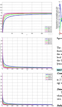
Figure 1. Numerical solution of system (1) for equilibrium point E1 with different values: α= 0.6, α = 0.7, α = 0.8 and

α = 0.9

the order of fractional while Rida et al. [14] modified the eco-epidemiology model as a fractional eco-epidemiolog-ical model. Model assumed the population of predators and prey populations affected by disease and predation is assumed to follow Holling-type I functional response.

In this article, we modify the eco-epidemiological model proposed by Saifuddin et al. [7]. It is assumed that the growth rate of the three populations not only depend on the current conditions but also take into con-sideration all previous state. Therefore, by changing the first order derivative into a fractional order derivative, the model proposed by Saifuddin et al. [7] will be mod-ified into a fractional order eco-epidemiological model.

Figure 2. Numerical solution of system (1) for equilibrium point with α= 0.74

The paper investigates the dynamics of the obtained fractional order eco-epidemiological model. We present the existence of equilibrium points and investigate the local asymptotic stability. The model is simulated using the Grünwald-Letnikov approximation to support ana-lytical results.

MATERIALS AND METHODS

Construction model

At this stage, the eco-epidemiology model proposed in [7] is modified into a fractional order eco-epidemiol-ogy model.

Determination of the equilibrium point

The equilibrium point of the system is obtained when the growth rate of populations is unchanged or zero.

Stability analysis of the equilibrium point

The local stability of the equilibrium point can be determined by the absolute value of the argument eigen-values of the Jacobian matrix equilibrium. The condition stability shows whether the equilibrium point is stable or not. If the equilibrium point is stable, then any solu-tion of the system with different initial values will be convergent to it, and vice versa.

Numerical experiments

(3)

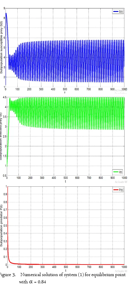
Figure 3. Numerical solution of system (1) for equilibrium point with α= 0.84

RESULTS AND DISCUSSION

Mathematical model

A fractional order eco-epidemiological model intro-duces by changing the first derivative into some frac-tional order Caputo-type derivatives. Suppose (S) is the susceptible prey population, (I) is the infected prey pop-ulation and (P) is the predator poppop-ulation. We assume the three population densities depend on all previous state.

Susceptible prey dynamic moves exponentially to-wards carrying capacity, while carrying capacity is the ratio of the growth rate (r) with intra-class competition

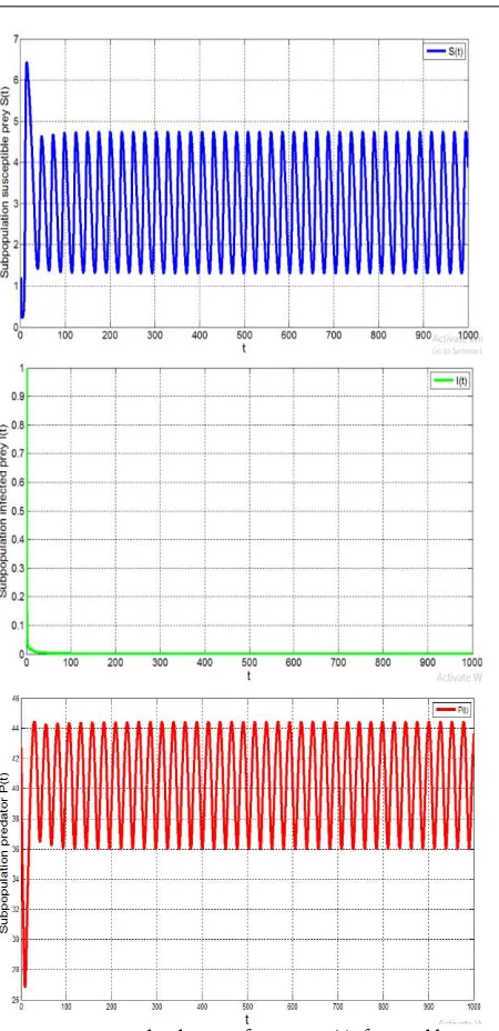
Figure 4. Numerical solution of system (1) for equilibrium point E3 with α= 0.74

in susceptible prey (b). Saifuddin et al. [7] assume, the infected prey is not in a state to produce but to compete with susceptible for the same resources. Interclass com-petetion between susceptible prey and infected prey (c) reduces the population growth rate. Contact between susceptible prey and infected prey causes susceptible prey become infected, where is the rate of infection of the disease, and a is the half saturation constant for the disease transmission. Infected prey density is reduced due to the death of infected prey. The death rate of in-fected prey is assumed to be .

Predator population consume both susceptible and infected prey with Holling type II functional response. Assume that 1 is the attack rate of predator on suscep-tible prey, 2 is the attack rate of predator on infected prey, c1 and c2 are the conversion efficiency of predator,

e is the half-saturation constant of predator for

suscep-tible prey, d is the half-saturation constant of predator for infected prey and

m is the death rate of predator.

Then we obtain the following fractional order system:

𝑑𝛼_𝑆

𝑑𝑡𝛼 = (𝑟 − 𝑏𝑆) − 𝑐𝐼𝑆 −_{𝑎 + 𝑆 −}𝛽𝐼𝑆 𝛼_{𝑒 + 𝑆}1𝑃𝑆

𝑑𝛼_𝐼

𝑑𝑡𝛼=

𝛽𝑆𝐼 𝑎 + 𝑆 −

𝛼2𝑃𝑆

𝑑 + 𝐼 − 𝜇𝐼, 𝑑𝛼_𝑃

𝑑𝑡𝛼 =

𝑐1𝛼1𝑆𝑃

𝑒 + 𝑆 − 𝑐2𝛼2𝐼𝑃

𝑑 + 𝐼 − 𝑚𝑃,

(1)

Equilibrium point

The equilibria of the system (1) are solutions to the system:

𝑑𝛼_𝑆

𝑑𝑡𝛼 =

𝑑𝛼_𝐼

𝑑𝑡𝛼 =

𝑑𝛼_𝑃

𝑑𝑡𝛼 = 0

(4)

𝑏

3. 𝐸2= (_𝛽−𝜇𝜇𝑎 ,_{(𝛽−𝜇)(𝑐𝑎+𝛽−𝜇)}𝑎[𝑟(𝛽−𝜇)−𝑏𝜇𝑎], 0), as the survival of both

susceptible and infected prey,

4. 𝐸3= (_𝑐₁_𝛼𝑚𝑒₁_−𝑚, 0,𝑐1𝑒(𝑐_(𝑐1𝛼₁1_𝛼𝑟−𝑟𝑚−𝑏𝑚𝑒₁_−𝑚)2 , ), as the infected

prey free equilibria,

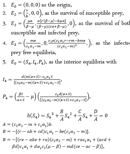
5. 𝐸0= (𝑆4, 𝐼4, 𝑃4), as the interior equilibria with

𝐼4=_[(𝑐 𝑑(𝑚(𝑒+𝑆)−𝑐1𝛼1𝑆

2𝛼2−𝑚)(𝑒+𝑆)+𝑐1𝛼1−𝑆],

𝑃4= (_𝑎+𝑆𝛽𝑆 − 𝜇) (_[(𝑐₂_𝛼₂_{−𝑚)(𝑒+𝑆)+𝑐}𝑐2𝑑(𝑒+𝑆) ₁_𝛼₁_−𝑆]),

ℎ(𝑆4) = 𝑆43+𝐵_{𝐴 𝑆}42+𝐶_{𝐴 𝑆}4+𝐷_{𝐴 = 0}

𝐴 = (𝑐2𝛼2− 𝑚 + 𝑐1𝛼1)𝑏,

𝐵 = −[(𝑟 − 𝑎𝑏 + 𝑐𝑑)𝑐1𝛼1− 𝑏𝑒(𝑐2𝛼2− 𝑚)],

𝐵 = −[(𝑟𝑒 − 𝑎𝑏𝑒 + 𝑟𝑎)(𝑐2𝛼2− 𝑚) + 𝑟𝑎𝑐1𝛼1+ (𝑎𝑐𝑑 +

𝛽𝑑)𝑐1𝛼1+ 𝑑𝛼1𝑐2(𝜇 − 𝛽) − 𝑚𝑑(𝑐𝑒 − 𝑎𝑐 − 𝛽)],

Stability of equilibrium point

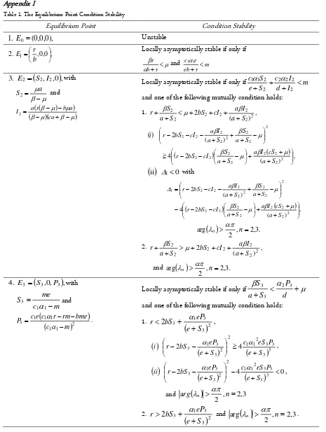
The dynamical behavior of system (1) around each equilibrium point can be studied by investigating the lo-cal stability of the equilibrium point. The lolo-cal stability is determined by the eigenvalues (λ) of the Jacobian ma-trix evaluated at the equilibrium point. The equilibrium point is stable if all eigenvalues satisfy |arg(λ)| > α π/2. It is found that equilibrium E0 = (0, 0, 0) is unstable node, which implies that all population will never go to extinct. Other equilibrium points are conditionally sta-ble. The stability conditions of equilibrium points for system (1) are summarized in appendix.

Numerical simulations

In this section, some numerical simulations are given to illustrate the analysis results and show the ef-fects of fractional order of the system. We run four sim-ulations.

The parameters used in the first simulation are

r = 3, b = 0.3, c = 0.1, a = 0.5,

β = 1.5, α1= 0.3, e = 3, α2

= 0.1, d = 3, µ = 1.8, c1 = 0.8, and m = 0.8. Based on these parameters, it is found that there are two equilibrium points namely E0(0,0,0) and E1(0,0,0). It is noted that

𝛽𝑟

𝑎𝑏+𝑟= 1.43 < 𝜇 = 1.8 and 𝑐1𝛼1𝑆2

𝑒𝑏+𝑟 = 0.16 < 𝑚 = 0.8.

Ac-cording Table 1, E1 is asymptotically stable irrespective of α while E0 is unstable.

The numerical simulation of this case with α= 0.6,

convergence of solutions to the equilibrium point E1. In this simulation, the relatively high values of death rate of infected prey and predator causes the extinction of infected prey and predator. Furthermore, the survival of susceptible prey is supported by the environment with carrying capacity (r / b).

Secondly, we set the same parameter as before ex-cept for

µ = 1.3. We obtain three positive equilibrium

points, namely

E

0 = (0,0,0),

E

1 = (10,0,0), and

E

2 =

(3.25,4.05,0). Based on these parameters, it is found that

𝑐1𝛼1𝑆2

𝑒+𝑆2 +

𝑐2𝛼2𝐼2

𝑒+𝐼2 = 0.16 < 𝑚 = 0.8 and 𝑟 +

𝛽𝑆2

𝑎+𝑆2= 4.3 >

𝜇 + 2𝑏𝑆2+ 𝑐𝐼2+_(𝑎+𝑆𝑎𝛽𝐼₂2₎2= 3.87 . Furthermore, we have

|arg(λ)| = 1.2 and α*

= 0.76. According to the condition

in Table 1, if we take α

= 0.74 then |arg(

λ)| = 1.2 >𝑎𝜋₂ = 1.16, which satisfies condition (ii), therefore E2 is asymp-totically stable. Figure 2 shows that the solution of sys-tem (1) is convergent to

E

2. It shows that the system goes to the co-existence of susceptible prey and infected prey, while the predator goes to extinction.

However, as seen in Figure 3, if we take α = 0.84 then |arg(λ)| = 1.2 < απ/2 = 1.32. Hence, the equilib-rium point E2 is unstable. In this case, the system shows a periodic behavior. Biologically, if the predation rate is smaller than the death rate of predator, then the preda-tor population cannot survive. On the other hand, the relatively small death rate of infected prey can cause the infected prey densities increased asymptotically. Figure 2 and 3 show that the variation of α causes changing the population densities. If α < α* then the population den-sities are convergent to E2 while if α > α* then the pop-ulation densities become fluctuation.

For the third simulation, we consider the same parame-ter values as in the second simulation, except for m = 0.1 We have four positive equilibrium points, namely

E

0(0,0,0),

E

1(10,0,0),

E

2(3.25,4.05,0), and

E

3(2.73,0,41.65). In this case we have _𝑎+𝑆𝛽𝑆3

3= 0.7 <

𝛼2𝑃3

𝑑 +

𝜇 = 2.6 and 𝑟 = 3 > 2𝑏𝑆3+_(𝑎+𝑆𝛼2𝑒𝑃₃3₎2= 2.8. We also have

(5)

Figure 5. Numerical solution of system P(t) for equilibrium point E3 with α= 0.85

Figure 5 illustrates solution for the case of α = 0.84, we have |arg(λ)| = 1.24 > απ/2 = 1.32. Consequently, equilibria is unstable because its stability condition is not satisfied. This behavior is depicted in Figure 5 which shows that both susceptible prey and predator popula-tions exhibit periodic oscillation and do not converge to equilibrium point E3(2.73,0,41.65). From Figure 4 and 5 we conclude that if α < α* then E3 is locally asymptoti-cally stable and vice versa.

From the ecological point, a relatively low infection rate causes the disease-free population. Furthermore, a relatively small death rate of predator will support the survival of predator population.

Figure 6. Numerical solution of system (1) for equilibrium point E4 with α= 0.65

Finally, we perform simulation using the same parameter as in Simulation 1, except α2 = 1.5 and µ = 1.3.

We have four positive equilibrium points,

E

0(0,0,0),

E

1(10,0,0),

E

2(3.25,4.05,0), and

E

3(5.8,3.69,0.37). Here we have b1 = 0.88, b2 = 0.12, b3 = 0.01, and D(P) = -0.02 < 0, then with α = 0.65, condition (ii) is satisfied and E4 locally asymptotically stable. The numerical simulation in Figure 6 shows that solution of system (1) with initial condition

S(0) = 5, I(0) = 3, and

P(0) = 1 and is

con-vergent to (5.8,3.69,0.37).

The increased attack rate on infected prey (α2) re-duces the infected prey densities and increases the pred-ator population.

CONCLUSION

In this paper, we have studied a fractional order eco-epidemiological model. It is found that the model has five equilibrium points, i.e., the origin, the survival of susceptible prey, the predator free equilibria, the in-fected prey free equilibria and the interior equilibria. Numerical results show the same result with analysis. It has been found E0 is always unstable, and the others

are locally asymptotically stable under some conditions. Numerical simulations indicate fractional order α is a factor which affects the behavior of solutions. There ex-ists α* > 0 such that if αϵ [0, α*) the equilibrium point is asymptotically stable and the population densities be-come stationary. If α* < α, then the equilibrium point becomes unstable and both prey and predator popula-tion show a fluctuapopula-tion behavior.

ACKNOWLEDGMENT

(6)

REFERENCES

1. Brauer F, Castillo-Chavez C (2011) Mathematical models in population biology and epidemiology. 2nd Edition. New York, Springer.

2. Rosenzweig ML, MacArthur RH (1963) Graphical represen-tation and stability condition of predator-prey interactions. American Naturalist 97 (895): 209 – 223. doi: 10.1086/282272.

3. Hadeler KP, Freedman HI (1989) Predator-prey populations with parasitic infection. Journal of Mathematical Biology 27 (6): 609 – 631. doi: 10.1007/BF00276947.

4. Suryanto A (2017) Dynamics of an eco-epidemiological model with saturated incidence rate, AIP Conference Proceedings 1825: 020021. doi: 10.1063/1.4978990. 5. Chattopadhyay J, Arino O (1999) A Predator-prey model

with disease in the prey. Nonlinear Analysis: Theory, Meth-ods and Applications 36 (6): 747 – 766. doi: 10.1016/S0362-546X(98)00126-6.

6. Saifuddin Md, Sasmal SK, Biswas S et al. (2015) Effect of emergent carrying capacity in an eco-epidemiological sys-tem. Mathematical Methods in the Applied Sciences 39 (4): 806 – 823. doi: 10.1002/mma.3523.

7. Saifuddin Md, Biswas S, Samanta S et al. (2016) Complex dynamics of an eco-epidemiological model with different competition coefficients and weak alle in the predator.

8. Diethelm K (2010) The analysis of fractional differential equations. Berlin, Springer-Verlag.

9. Petras I (2011) Fractional-order nonlinear systems: Model-ing, analysis and simulation Berlin, Springer-Verlag. doi: 10.1007/978-3-642-18101-6.

10. Rihan FA, Lakshmanan S, Hashish AH et al. (2015) Frac-tional-order delayed predator-prey systems with Holling type-II functional response. Nonlinear Dynamics 80 (1 – 2): 777 – 789. doi: 10.1007/s11071-015-1905-8.

11. Suryanto A, Darti I, Anam S (2017) Stability analysis of a fractional order modified Leslie-Gower model additive Allee effects. International Journal of Mathematics and Mathematical Sciences 2017 (2017). doi: 10.1155/2017/8273430.

12. Rivero M, Trujillo JJ, Vázquez L, Velasco MP (2011) Frac-tional dynamics of populations. Applied Mathematics and Computation 218 (3): 1089 – 1095. doi: 10.1016/j.amc.2011.03.017.

13. Ghaziani RK, Alidousti J, Eshkaftaki AB (2016) Stability and dynamics of fractional order Leslie-Gower prey predator model. Applied Mathematical Modelling 40 (3): 2075 – 2086. doi: 10.1016/j.apm.2015.09.014.

(7)