ASSESSMENT OF MULTIRESOLUTION SEGMENTATION FOR EXTRACTING
GREENHOUSES FROM WORLDVIEW-2 IMAGERY
M. A. Aguilar a, *, F. J. Aguilar a, A. García Lorca b, E. Guirado c, M. Betlej a, P. Cichon a, A. Nemmaoui a, A. Vallario d, C. Parente d,
a Dept. of Engineering, University of Almería, 04120 Almería, Spain - [email protected], [email protected], [email protected],
[email protected], [email protected]
b Dept. of Geography, University of Almería, 04120 Almería, Spain - [email protected] c Dept. of Biology and Geology, University of Almería, 04120 Almería, Spain – [email protected]
d Dept. of Sciences and Technologies, University of Naples “Parthenope”, 80143 Naples, Italy - [email protected],
Commission VII, WG VII/4
KEY WORDS: Segmentation, Multiresolution, Object Based Image Analysis, WorldView-2, Scale, Shape, Compactness, Local Variance
ABSTRACT:
The latest breed of very high resolution (VHR) commercial satellites opens new possibilities for cartographic and remote sensing applications. In this way, object based image analysis (OBIA) approach has been proved as the best option when working with VHR satellite imagery. OBIA considers spectral, geometric, textural and topological attributes associated with meaningful image objects. Thus, the first step of OBIA, referred to as segmentation, is to delineate objects of interest. Determination of an optimal segmentation is crucial for a good performance of the second stage in OBIA, the classification process. The main goal of this work is to assess the multiresolution segmentation algorithm provided by eCognition software for delineating greenhouses from WorldView-2 multispectral orthoimages. Specifically, the focus is on finding the optimal parameters of the multiresolution segmentation approach (i.e., Scale, Shape and Compactness) for plastic greenhouses. The optimum Scale parameter estimation was based on the idea of local variance of object heterogeneity within a scene (ESP2 tool). Moreover, different segmentation results were attained by using different combinations of Shape and Compactness values. Assessment of segmentation quality based on the discrepancy between reference polygons and corresponding image segments was carried out to identify the optimal setting of multiresolution segmentation parameters. Three discrepancy indices were used: Potential Segmentation Error (PSE), Number-of-Segments Ratio (NSR) and Euclidean Distance 2 (ED2).
* Corresponding author
1. INTRODUCTION
The latest very high resolution (VHR) commercial satellites successfully launched over the past years (e.g., GeoEye-1, WorldView-2 and WorldView-3) are being the focus of intensive research in the remote sensing field. VHR satellite images are being increasingly used for different land use/land cover detection and classification. Most of these research works were conducted using object based image analysis (OBIA) techniques (Carleer and Wolff, 2006; Stumpf and Kerle, 2011; Pu et al., 2011; Pu and Landry, 2012; Aguilar et al., 2013; Fernández et al., 2014; Heenkenda et al., 2015).
OBIA techniques are based on aggregating similar pixels to obtain homogenous objects, which are then assigned to a target class. Using objects instead of pixels as a minimum unit of information minimizes the salt and pepper effect due to the spectral heterogeneity of individual pixels. Furthermore, and unlike traditional pixel-based methods that only use spectral information, object-based approaches can use shape, texture, and context information associated with the objects and thus have the potential to efficiently handle more difficult image analysis tasks (e.g. Marpu et al., 2010). A comprehensive review of the advantages and disadvantages of using OBIA techniques for image classification, as well as the state of the art
of these methods, can be found in Blaschke (2010) and Blaschke et al. (2014).
The first stage in OBIA is the image segmentation. This crucial process splits an image into separated non-overlapping homogeneous regions. This step is decisive because the resulting image segments form the basis for the subsequent classification (Blaschke, 2010; Witharana and Civco, 2014). There exist several types of image segmentation algorithms developed for a variety of applications in various fields of image analysis. Most of them largely depend on specified parameters, implying that segmentation is not an easy task. At this point, it should be clearly stated that much of the work referred to as OBIA has been originated around the software eCognition. Indeed, about 50–55% of the papers related to OBIA used this software package (Blaschke 2010). In this way, eCognition Developer’s proprietary multiresolution segmentation (Baatz and Schäpe, 2000) has proven to be one of the most successful image segmentation algorithms in the OBIA framework (Neubert et al., 2008). Scale, Shape, and Compactness are the main parameters available to users that affect the performance of the algorithm.
Different combinations of these parameters may produce different segmentation results. The selection of the optimal
value combination is often a tedious trial-and-error process. To help the user with the selection of these parameters, unsupervised methods based on the local variance such as Estimation of Scale Parameters tool for a single band (ESP tool) (Dragut et al., 2010) and for multiband images (ESP2 tool) (Dragut et al., 2014) have been proposed. Also, supervised methods based on the measure of dissimilarity between segmentation results and user-generated (e.g., hand digitized) reference objects have been used to identify the optimal combination of parameter values among all examined combinations (e.g., Clinton et al., 2010; Liu et al., 2012).
Automatic mapping of greenhouses from remote sensing methods presents a special challenge due to their unique characteristics. The first work using eCognition and multiresolution segmentation for plastic greenhouse detection was published by Tarantino and Figorito (2012). They used digital true colour (RGB) aerial data in different study areas of Italy. The optimal segmentation parameters (300, 0.5 and 0.8 for Scale, Shape and Compactness respectively) were attained by applying a trial-and-error approach. In the other two OBIA studies dealing with greenhouse detection from VHR satellite imagery (Aguilar et al., 2014; Aguilar et al., 2015), the segmented objects were generated by manual digitizing, thus avoiding the problems related to segmentation stage (e.g. the setting of multiresolution segmentation parameters).
In this work, segmentation stage is faced by estimating the optimal parameters approach (i.e., Scale, Shape and Compactness) of the multiresolution segmentation algorithm included into eCognition software for delineating plastic greenhouses in OBIA environment from WorldView-2 multispectral orthoimages. To the best knowledge of the authors, this is the first research work dealing with this topic on very high resolution satellite images.
2. STUDY SITE AND DATASETS 2.1 Study site
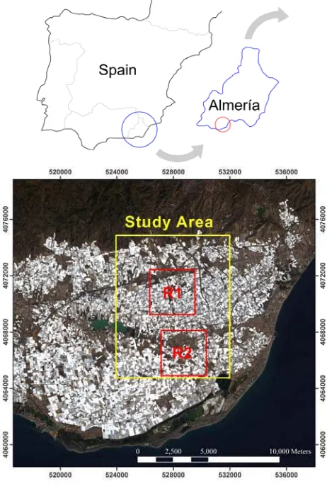
This investigation was conducted in Almería, southern Spain, which has become the site of the greatest concentration of greenhouses in the world, known as the “Sea of Plastic”. The study area comprised a rectangle area of about 8000 ha centered on the WGS84 geographic coordinates of 36.7824°N and 2.6867°W (Fig. 1). Inside the study area, two square subareas or repetitions (R1 and R2) with sides of 3200 m were extracted.
2.2 WorldView-2 Data
WorldView-2 (WV2) is a VHR satellite launched in October 2009. This sensor is capable of acquiring optical images with 0.46 m and 1.84 m ground sample distance (GSD) at nadir in panchromatic (PAN) and multispectral (MS) mode, respectively. Moreover, it was the first VHR commercially available providing 8 band MS satellite: coastal (C, 400-450 nm), blue (B, 450-510 nm), green (G, 510-580 nm), yellow (Y, 585-625 nm), red (R, 630-690 nm), red edge (RE, 705-745 nm), near infrared-1 (NIR1, 760-895 nm) and near infrared-2 (NIR2, 860-1040 nm).
A single WV2 image taken on 30 September 2013 over the study area was acquired. It was collected in Ortho Ready Standard Level-2A (ORS2A) format, containing both PAN and MS imagery. This satellite image had a mean off-nadir view
angle of 11.8°, a mean collection azimuth of 38.2° and 0% of cloud cover. The final product GSD was of 0.4 m and 1.6 m for PAN and MS images respectively.
Figure 1. Location of the study area (yellow rectangle) and two subareas (red squares). Coordinate system: ETRS89 UTM 30N.
From this WV2 ORS2A bundle image, a pan-sharpened image with 0.4 m GSD was attained by means of the PANSHARP module included in Geomatica v. 2014 (PCI Geomatics, Richmond Hill, ON, Canada). The coordinates of seven ground control points (GCPs) and 32 independent check points (ICPs) were obtained by differential global positioning system (DGPS) using a total GPS Topcon HiPer PRO station working in real-time kinematic mode (RTK). The ground points (both GCPs and ICPs) were measured with reference to the European Terrestrial Reference System 1989 (ETRS89) and UTM Zone 30 projection. A pan-sharpened RGB orthoimage with 0.4 m GSD was generated by using the seven GCPs to compute the sensor model based on rational functions refined by a zero order transformation in the image space (RPC0). A medium resolution 10 m grid spacing DEM with a vertical accuracy of 1.34 m (root mean square error; RMSE), provided by the Andalusia Government, was used to carry out the orthorectification process. The planimetric accuracy (RMSE2D) attained on the orthorectified pan-sharpened image and measured through the 32 ICPs took a value of 0.59 m.
Furthermore, a MS orthoimage with 1.6 m GSD and containing the full 8-band spectral information was also produced. The same seven GCPs, RPC0 model and DEM were used to attain the MS orthoimage. As a prior step to the orthorectification
process, the original WV2 MS image was atmospherically corrected by using the ATCOR (atmospheric correction) module included in Geomatica v. 2014. Finally, an atmospherically-corrected WV2 MS orthoimage with a RMSE2D of 2.20 m was generated.
2.3 Reference Greenhouses
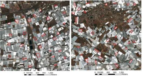
This work is focused on optimizing the plastic greenhouse delineation provided by the multiresolution segmentation included into eCognition software. In this way, only one land cover or class is studied. In each of the two subareas showed in Fig. 1 (R1 and R2), 30 greenhouses (60 greenhouses in total) were manually digitized working on the aforementioned WV2 pan-sharpened orthoimage. A similar number of polygons per class was also used in previous segmentation quality studies (Liu et al., 2012; Witharana and Civco, 2014). Figure 2 shows these digitized reference polygons presenting a variable size and shape for both subareas. The statistics related to the reference polygons are shown in Table 1.
Figure 2. Reference greenhouse polygons in red digitized on R1 (left) and R2 (right) subareas.
Subarea R1 Subarea R2
Number of Polygons 30 30
Total Area (m2) 274,115.5 249,115.7
Average Area (m2) 9,137.2 8,303.9
Maximum Area (m2) 21,077.0 14,951.4
Minimum Area (m2) 2,797.3 2,749.8
Standard Deviation (m2) 4,140.6 3,529.5
Table 1. Statistics from the reference polygons digitized on R1 and R2 subareas.
3. METHODOLOGY 3.1 Image segmentation
The image segmentation algorithm used in this research is the so-called multiresolution segmentation included into the OBIA software eCognition v. 8.7. This segmentation approach is a bottom-up region-merging technique starting with one-pixel objects. In numerous iterative steps, smaller objects are merged into larger ones (Baatz and Schäpe, 2000). But this task is not easy, and it highly depends on the desired objects to be segmented (Tian and Chen, 2007). The outcome of the multiresolution segmentation algorithm is controlled by three main factors: (i) the homogeneity criteria or scale parameter (SP) that determines the maximum allowed heterogeneity for the resulting segments, (ii) the weight of colour and shape criteria in the segmentation process (Shape), and (iii) the weight of the compactness and smoothness criteria (Compactness). The optimal determination of these three somewhat abstract terms is
not easy to carry out. However, a detailed review of the multiresolution segmentation algorithm is beyond the scope of this paper. More information about the mathematical formulation of multiresolution segmentation can be found in the literature (e.g., Baatz and Schäpe, 2000; Tian and Chen, 2007; Trimble Germany GmbH, 2011).
3.2 Scale Parameter (SP) determination
An unsupervised tool proposed by Dragut et al. (2014), called “Estimation of Scale Parameter 2” (ESP2), was used in this work to select the ideal multiresolution SP for each test. The ESP2 tool was programmed in CNL within the eCognition software environment. ESP2 automatically segments the user defined data with fixed increments of SP and calculates local variance (LV) as the mean SD of the objects for each object level obtained through multiresolution segmentation. This tool works in a similar way that the original ESP (Dragut et al., 2010), but ESP2 has been designed to be applied to multispectral images. Both ESP and ESP2 are based on the following hypothesis. When growing the size of a segment, its SD increases continuously up to the point that it matches the object in the real world. Assuming a certain amount of spectral contrast between the object and background, the object boundaries will be preserved in segmentation at a number of higher levels, where the SD of this object remains the same. In the same way, objects of similar size and spectral response are expected to match their correspondents in the real world around the same scale level. As such, their boundaries, and implicitly their SD values, will be conserved along a number of further coarser scale levels. If this type of object is well represented in the image, the cumulative effect of preserving the SD values of objects just above the meaningful scale level will be strong enough to impact upon the LV of that image. The optimal SP value can be automatically extracted at the point where the LV value at a given level (LVn) is equal to or lower than the previous value recorded at the level (LVn-1). The level n-1 would be then selected as the optimal scale for segmentation.
3.3 Segmentation quality metrics
Supervised segmentation quality metrics are focused on the scenario in which a set of training or reference objects (usually manually digitized) is available for an image, and segmentation results are to be compared to these predefined reference objects. In this work, and in order to assess the goodness of the different segmentations, the outputs were compared to 30 manually delineated reference polygons representing greenhouses (Fig. 2) for each one of the two working subareas (R1 and R2). This number of polygons was previously recommended by Liu et al. (2012).
Although there are several supervised methods and metrics to assess the goodness of segmentation (Zhang, 1996; Clinton et al., 2010), perhaps the supervised discrepancy measure known as Euclidean Distance 2 (ED2), recently proposed by Liu et al. (2012), is one that has shown better performance. In a nutshell, ED2 tries to optimize in a two dimensional Euclidean space both the geometrical discrepancy (by mean of the potential segmentation error (PSE)) and also the arithmetic discrepancy between image objects and reference polygons (by using the number-of-segmentation ratio (NSR)).
In order to compute ED2, Liu et al. (2012) defined the corresponding segment dataset. The corresponding segments can be extracted from each original segment dataset and only
contains those image segments that spatially overlap with the reference polygons. Moreover, two conditions called areal-overlap-based criteria have been used to effectively identify corresponding segments (Clinton et al., 2010): (i) All segments in an original segment dataset are candidates for this process. (ii) A candidate segment can be labelled as a “corresponding segment” if the area of intersection between a reference polygon and the candidate segment is more than half the area of either the reference polygon or the candidate segment.
Figure 3. Illustration of geometric discrepancies between reference polygons and candidate/corresponding segments on a
reference greenhouse from R1.
Figure 3 depicts the candidate and corresponding segments extracted from two multiresolution segmentations for the same reference greenhouse (polygon) belonging to the subarea R1. Segmentation showed in Figure 3a corresponds to 50, 0.1 and 0.5 values for SP, Shape and Compactness parameters respectively. A different set of parameters were used in Figure 3b (SP=62, Shape=0.9, Compactness=0.5). We can make out the main possible geometric discrepancies: over-segment, under-segment and overlapped area. ED2 measures the geometric discrepancies by means of PSE, which is defined as the ratio between the total area of under-segments and the total area of reference polygons (Eq. 1), where rk is the k-th reference polygon in the reference dataset or ground truth (k = 1, 2, . . ., m) and si represent the corresponding segments belonging to the candidates dataset associated to the i-th reference polygon (i = 1, 2, . . ., v). A PSE value of zero indicates that there are no under-segments. A large value implies a significant degree of under-segmentation.
However, although a geometric relationship is necessary, it may not be sufficient to describe the diverse types of discrepancy between reference and corresponding polygons. Hence arithmetic discrepancies are also included into ED2 metric through NSR index. It is defined as the absolute difference between the number of reference polygons (m) and the number of corresponding segments (v) divided by the number of reference polygons (Eq. 2).
m v m abs
NSR ( ) (2)
Finally, ED2 can be computed as a composite index that considers both geometric and arithmetic discrepancies (Eq. 3).
A point in a two-dimensional PSE–NSR space corresponds to the paired PSE and NSR value obtained from Eq. (1) and Eq. (2), respectively. indicates a combination of both a desirable geometric match and a desirable arithmetic match. A desirable geometric match is where there are no over-segments or under-segments. A desirable arithmetic match is where a reference polygon is in response to only one corresponding segment. A large ED2 value indicates either a significant geometric discrepancy, or a significant arithmetic discrepancy, or both.
3.4 Analysis workflow
Different combinations of Shape and Compactness parameters were tested in this work. Concretely, five values {0.1, 0.3, 0.5, 0.7, 0.9} were selected as alternative weights for both Shape and Compactness parameters, so meaning 25 possible combinations. These same values for Shape and Compactness parameters were tested by Kavzoglu and Yildiz (2014) in an assessment of multiresolution segmentation over QuickBird and aerial orthoimages. For each one of these 25 combinations of parameters, the ESP2 tool (Dragut et al., 2014) was run into eCognition over the R1 and R2 subareas covered by the 8-band WV2 MS orthoimage. The ESP2 setting values were kept the same for every combination, taking the following values: non-hierarchy option, starting scale level 1 = 10, step size level 1 = 1 and number of loops = 90 (Fig. 4). It is important to note that the second and third ESP2 levels in our study applied step sizes of 5 and 10 respectively. Those second and third levels produced segments much larger than a single greenhouse, so only level 1 was considered. Thus, ESP2 provided 25 segmentation results for each one of the two working subareas (i.e. 50 segmentation results).
Figure 4. The graphical user interface of ESP2. The setting values used in the tests are described for different combinations
of Shape and Compactness (in this case Shape and Compactness were fixed to 0.1 and 0.9 respectively).
4. RESULTS AND DISCUSSION
Table 2 shows the SP and ED2 values attained for each of the 25 combinations of parameters (Shape and Compactness) used in both study areas (R1 and R2).
Regarding the SP value computed by ESP2 tool (Dragut et al., 2014), the application of LV to find the optimal SP in the multiresolution segmentation algorithm applied to segment greenhouses (WV2 MS orthoimage) achieved acceptable results. The fact that the greenhouses under study presented a very similar shape and size, together with they occupied most of the study area, worked to the good performance of ESP2 tool. Although SP values were ranging from 24 to 86, the most frequent values were usually quite grouped in the case of the best segmentations (SP values between 45 and 55). On the other hand, time is an important factor when assessing the performance of a tool. The processing times were around of 2 hours for each project on a 2000 pixel by 2000 pixel subarea using a laptop PC equipped with INTEL® CORE™ i5 CPU 460M, 2.53 GHz and 4 GB RAM.
Concerning the ED2, slightly better values were attained in R2 subarea. This probably was due to the fact that the reference greenhouses digitized in R2 area were more homogeneous than the ones delineated in R1 (Table 1). However the final SD and average statistic values depicted in Table 2 turned out to be very similar in both subareas.
Shape Compactness R1 R2
SP ED2 SP ED2
0.1 0.1 55 0.34 50 0.09
0.1 0.3 55 0.23 49 0.18
0.1 0.5 50 0.19 52 0.08
0.1 0.7 55 0.17 55 0.08
0.1 0.9 38 0.53 48 0.21
0.3 0.1 42 0.29 48 0.24
0.3 0.3 64 0.41 52 0.11
0.3 0.5 53 0.16 47 0.08
0.3 0.7 45 0.13 57 0.13
0.3 0.9 42 0.15 49 0.15
0.5 0.1 50 0.21 35 0.27
0.5 0.3 51 0.22 47 0.04
0.5 0.5 47 0.14 42 0.18
0.5 0.7 66 0.37 43 0.30
0.5 0.9 54 0.31 44 0.34
0.7 0.1 51 0.21 38 0.06
0.7 0.3 51 0.26 52 0.11
0.7 0.5 51 0.45 79 1.15
0.7 0.7 62 0.78 66 1.09
0.7 0.9 43 0.78 24 2.97
0.9 0.1 72 2.62 46 0.41
0.9 0.3 75 2.65 66 1.74
0.9 0.5 62 1.17 86 3.08
0.9 0.7 82 2.65 63 1.09
0.9 0.9 68 1.19 72 1.84
Max 82 2.65 86 3.08
Min 38 0.13 24 0.04
SD 11.0 0.80 13.67 0.89 Average 55.3 0.66 52.4 0.64 Table 2. Values and statistics for Euclidean Distance 2 (ED2)
according to each combination of Shape, Compactness and scale parameter (SP computed with ESP2 tool) for both R1 and
R2 study subareas.
(a) Ortho VW2 MS (b) ED2 = 0.19; SP = 50; SH =0.1
(c) ED2 = 0.16; ; SP = 53; SH =0.3 (d) ED2 = 0.14; SP = 47; SH =0.5
(e) ED2 = 0.45; SP = 51; SH =0.7 (f) ED2 = 1.17; SP = 62; SH =0.9
Figure 5. Details of segmentation results (green polygons) for different parameter combinations as compared to reference greenhouses (red polygons). Compactness was kept constant as
0.5, while scale parameter (SP) was computed by ESP2 tool. The Shape parameter took varying values (SH = 0.1, 0.3, 0.5,
0.7, 0.9).
Figure 5 shows the graphical representation of some segmentation results for the subarea R1. It can be appreciated that the best segmentations, both visually and according to the ED2 value, were attained for Shape parameters ranging from 0.1 to 0.5 (Fig. 5b, Fig. 5c and Fig. 5d). In these three cases the SP computed by ESP2 tool was found to be pretty consistent (50, 53 and 47 respectively). Moreover, the segmentations with Shape of 0.7 and 0.9 (Fig. 5e and Fig. 5f) presented the highest discrepancy between segment (green) and reference polygons (red). For Shape parameters of 0.1, 0.3 and 0.5, there were tiny differences in ED2 values, all of them provided very good results as compared to with the reference greenhouses. However, and applying a subjective visual analysis over the whole of greenhouses shown in Figure 5 (not only the reference ones in red), the best segmentation seems to be depicted in Figure 5c (Shape = 0.3) closely followed by the results shown in Figure 5b (Shape = 0.1). In short, the slightly differences observed in ED2 values could be due to the reference polygons
selected. The results obtained from using the Shape parameter of 0.5 were slightly worse than those achieved for 0.1 or 0.3 Shape values in subarea R1 and, especially, in subarea R2.
Figure 6 shows the evolution in both tests (R1 and R2, i.e., 50 repetitions) of NSR (Fig. 6a), PSE (Fig. 6b) and ED2 (Fig. 6c) with SP. SP turns out to be, without any doubt, the most important parameter controlling multiresolution segmentation (Dragut et al., 2014). All figures are showing their third-degree polynomial trendlines and the corresponding coefficient of determination (R2). It can be easily seen that ED2 presented a pronounced minimum value close to 47. This finding indicates that ESP2 tool performed very well dealing with greenhouses and ED2 brilliantly highlighted the optimal SP values. The left branch of the ED2 trendline is mainly conducted by the NSR values (Fig. 6a), while the branch on the right is triggered mostly by PSE values (Fig. 6b). The shape of the ED2-SP scattergrams turned out to be very similar to the one reported by Liu et al. (2012) and Witharana and Civco (2014).
(a) (b)
(c)
Figure 6. Scattergrams showing the variation with scale parameter (SP) of number-of-segmentation ratio (NSR) (a), potential segmentation error (PSE) (b) and Euclidean distance 2
(ED2) (c), for R1 and R2 subareas.
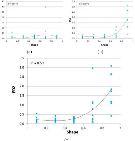
Figure 7 displays the evolution of NSR (Fig. 7a), PSE (Fig. 7b) and ED2 (Fig. 7c) according to the variation of the Shape parameter. Looking at R2 values, the influence of Shape in ED2 metric was lower than for SP. The Shape parameter had no effect on NSR values, though it influenced on PSE values. Overall, PSE tended to increase (i.e., more under-segmentation error) when increasing the Shape parameter. This trend for PSE was also reflected by ED2. In this sense, values of Shape parameter higher than 0.5 (that is penalizing spectral information or colour) should be avoided for plastic greenhouses segmentation.
Figure 8 shows the variation of NSR (Fig. 8a), PSE (Fig. 8b) and ED2 (Fig. 8c) values in relation to the Compactness parameter. R2 values for these charts evinced no relationship
between Compactness parameter and any of the three goodness segmentation metrics tested. As a result, it was assumed that the Compactness parameter did not have considerable effect in the creation of meaningful greenhouse objects. In fact, and reviewing the specialized literature, the weight of Compactness parameter has been generally set to a fix value of 0.5 by researchers (Liu and Xia, 2010; Dragut et al., 2014; Kavzoglu and Yildiz, 2014).
(a) (b)
(c)
Figure 7. Scattergrams showing the variation with shape of of number-of-segmentation ratio (NSR) (a), potential segmentation error (PSE) (b) and Euclidean distance 2 (ED2) (c), for R1 and R2 subareas.
(a) (b)
(c)
Figure 8. Scattergrams showing the variation with compactness of number-of-segmentation ratio (NSR) (a), potential segmentation error (PSE) (b) and Euclidean distance 2 (ED2) (c), for R1 and R2 subareas.
5. CONCLUSIONS
As far as we know, this work is the first attempt to identify the optimal values of the well-known multiresolution segmentation algorithm (i.e., SP, Shape and Compactness parameters) working on a plastic greenhouse area through an 8-band multispectral WV2 orthoimage. Setting of optimal values of segmentation is not an easy task, but it is crucial to achieve a successful classification in the context of an object based image analysis. Although this work should be only considered as a first approach, the following conclusions can be drawn:
1.- ESP2 tool worked quite well on plastic greenhouses multiresolution segmentation, estimating correct values for the SP parameter. The very similar shape and size of the greenhouses located at the study area likely positively influenced the good performance of ESP2 tool. The SP values obtained through ESP2 which visually performed very poor segmentation results (outliers) were related to the higher values of the Shape parameter (0.7 and specially 0.9).
2.- ED2 metric presented a very good relationship with the visual quality of the greenhouse segmentations. This measure was clearly related to SP and Shape, but had no relationship with Compactness.
3.- The ideal settings for delineating plastic greenhouses from 8-band multispectral WV2 orthoimages through eCognition multiresolution segmentation would be the followings: SP ranging from 45 to 55 and Shape parameter close to 0.3 (i.e., 0.1, 0.3, 0.5). Compactness parameter could be fixed to 0.5 according with our results and the reviewed literature. Summing up, the recommended way to compute these segmentation settings could be based on obtaining the SP parameter from the ESP2 tool by fixing the Compactness in 0.5 and testing two values for Shape (0.1 and 0.3).
ACKNOWLEDGEMENTS
This work was supported by FEDER funds and the Spanish Ministry of Economy and Competitiveness, the Spanish Government (AGL2014-56017-R). This is part of the general research lines promoted by the Agrifood Campus of International Excellence ceiA3 (http://www.ceia3.es/).
REFERENCES
Aguilar, M.A., Saldaña, M.M., Aguilar, F.J., 2013. GeoEye-1 and WorldView-2 pan-sharpened imagery for object-based classification in urban environments. International Journal of Remote Sensing, 34(7), pp. 2583-2606.
Aguilar, M.A., Bianconi, F., Aguilar, F.J., Fernández, I., 2014. Object-based greenhouse classification from GeoEye-1 and WorldView-2 stereo imagery. Remote Sensing, 6, pp. 3554-3582.
Aguilar, M.A., Vallario, A., Aguilar, F.J., García Lorca, A., Parente, C., 2015. Object-Based Greenhouse Horticultural Crop Identification from Multi-Temporal Satellite Imagery: A Case Study in Almeria, Spain. Remote Sensing, 7, pp. 7378-7401.
Baatz, M., Schäpe, M., 2000. Multiresolution segmentation - An optimization approach for high quality multi-scale image segmentation. In: Strobl, J., Blaschke, T., Griesebner, G. (Eds.),
Angewandte Geographische Informations-Verarbeitung XII. Wichmann Verlag, Karlsruhe, pp. 12-23.
Blaschke, T., 2010. Object based image analysis for remote sensing. ISPRS Journal of Photogrammetry and Remote Sensing, 65(2010), pp. 2-16.
Blaschke, T., Hay, G.J., Kelly, M., Lang, S., Hofmann, P., Addink, E., Feitosa, R.Q., van der Meer, F., van der Werff, H., van Coillie, F., Tiede, D., 2014. Geographic Object-Based Image Analysis—Towards a new paradigm. ISPRS Journal Photogrammetry and Remote Sensing, 87(2014), pp. 180-191.
Carleer, A.P., Wolff, E., 2006. Urban land cover multi-level region-based classification of VHR data by selecting relevant features. International Journal of Remote Sensing, 27(6), pp. 1035-1051.
Clinton, N., Holt, A., Scarborough, J., Yan, L., Gong, P., 2010. Accuracy assessment measures for object-based image segmentation goodness. Photogrammetric Engineering and Remote Sensing, 76 (3), pp. 289-299.
Dragut, L., Tiede, D., Levick, S., 2010. ESP: a tool to estimate scale parameters for multiresolution image segmentation of remotely sensed data. International Journal of Geographical Information Science, 24(6), pp. 859-871.
Dragut, L., Csillik, O., Eisank, C., Tiede, D., 2014. Automated parameterisation for multi-scale image segmentation on multiple layers. ISPRS Journal Photogrammetry and Remote Sensing, 88(2014), pp. 119-127.
Fernández, I., Aguilar, F.J., Aguilar, M.A., Álvarez, M.F., 2014. Influence of data source and training size on impervious surface areas classification using VHR Satellite and aerial imagery through an object-based approach. IEEE Journal of Selected Topics in Applied Earth Observations and Remote Sensing, 7(12), pp. 4681-4691.
Heenkenda, M.K., Joyce, K.E., Maier, S.W., 2015. Mangrove tree crown delineation from high-resolution imagery. Photogrammetric Engineering and Remote Sensing, 81(6), pp. 471-479.
Kavzoglu, T., Yildiz, M., 2014. Parameter-Based Performance Analysis of Object-Based Image Analysis Using Aerial and QuikBird-2 Images. ISPRS Annals of Photogrammetry, Remote Sensing and Spatial Information Sciences, II-7, pp. 31-37.
Marpu, P. R., Neubert, M., Herold, H., Niemeyer, I., 2010. Enhanced Evaluation of Image Segmentation Results. Journal of Spatial Science, 55(1), pp. 55-68.
Neubert, M., Herold, H., Meinel, G., 2008. Assessing image segmentation quality –concepts, methods and application. In: Blaschke, T., Hay, G., & Lang, S. (Eds.), Object-Based Image Analysis – Spatial Concepts for Knowledge-Driven Remote Sensing Applications. Lecture Notes in Geoinformation & Cartography 18, Berlin, Springer, pp. 769–784.
Liu, D., Xia, F., 2010. Assessing object-based classification: Advantages and limitations. Remote Sensing Letters, 1(4), pp.187-194.
Liu, Y., Biana, L., Menga, Y., Wanga, H., Zhanga, S., Yanga, Y., Shaoa, X., Wang, B., 2012. Discrepancy measures for selecting optimal combination of parameter values in object-based image analysis. ISPRS Journal of Photogrammetry and Remote Sensing, 68(2012), pp. 144-156.
Pu, R., Landry, S., Yu, Q., 2011. Object-based urban detailed land cover classification with high spatial resolution IKONOS imagery. International Journal of Remote Sensing, 32(12), pp. 3285-3308.
Pu, R., Landry, S., 2012. A comparative analysis of high spatial resolution IKONOS and WorldView-2 imagery for mapping urban tree species. Remote Sensing of Environment, 124(2012), pp. 516-533.
Stumpf, A., Kerle, N., 2011. Object-oriented mapping of landslides using Random Forests. Remote Sensing of Environment, 115(2011), pp. 2564-2577.
Tarantino, E., Figorito, B., 2012. Mapping rural areas with widespread plastic covered vineyards using true color aerial data. Remote Sensing, 4, pp. 1913-1928.
Tian, J., Chen, D.M., 2007. Optimization in mult-scale segmentation of high resolution satellite images for artificial feature recognition. International Journal of Remote Sensing, 28(20), pp. 4625-4644.
Trimble Germany GmbH, 2011. eCognition Developer 8.7 Reference Book, Trimble Germany GmbH, Germany.
Witharana, C., Civco, D.L., 2014. Optimizing multi-resolution segmentation scale using empirical methods: exploring the sensitivity of the supervised discrepancy measure Euclidean distance 2 (ED2). ISPRS Journal Photogrammetry and Remote Sensing, 87(2014), pp. 108-121.
Zhang, Y.J., 1996. A survey on evaluation methods for image segmentation. Pattern Recognition, 29(8), pp.1335-1346.
Revised February 2016