www.elsevier.comrlocateratmos
Precipitation in marine cumulus and stratocumulus.
Part I: Thermodynamic and dynamic observations
of closed cell circulations and cumulus bands
Jørgen B. Jensen
), Sunhee Lee, Paul B. Krummel, Jack Katzfey,
Dan Gogoasa
CSIRO Atmospheric Research, PMB 1, Aspendale, Victoria 3195, Australia
Received 28 June 1999; received in revised form 6 January 2000; accepted 8 February 2000
Abstract
A case study of vigorous drizzle development in marine boundary layer clouds is presented. The clouds were observed using a research aircraft west of Tasmania during the Southern Ocean
Ž
Cloud Experiment. A clean marine boundary layer contained both cumulus clouds some oriented
.
in bands and an upper level stratus deck organised in a closed cell circulation.
‘‘Cold pools,’’ that is regions of evaporatively cooled air under mature cumulus clouds, were observed on several occasions. Air in the cold pool centre showed a divergent component of the wind perpendicular to the mature cumulus bands. Ahead of this spreading precipitation downdraft, the wind component perpendicular to the cumulus band was convergent, and new cumulus clouds were subsequently formed over these regions.
This dynamical situation is likened to an actively developing squall line of the propagating type. The development of drizzle, and its evaporation in the mixed-layer below the base of mature cumulus bands, is critical to the cloud evolution. It is demonstrated here, that processes resembling ‘‘deep convection’’ may also be responsible for the cloud development in a marine boundary layer of only 1500 m depth.q2000 Elsevier Science B.V. All rights reserved.
Keywords: Stratocumulus; Precipitation; Cumulus; Boundary layer meteorology
)Corresponding author. Fax:q61-3-9239-4444.
Ž .
E-mail address: [email protected] J.B. Jensen .
0169-8095r00r$ - see front matterq2000 Elsevier Science B.V. All rights reserved.
Ž .
1. Introduction
Boundary-layer clouds span the entire spectrum between well-mixed stratocumulus clouds and isolated cumulus clouds. Often, stratocumulus and cumulus occur
simultane-Ž .
ously. Measurements from the North Sea Nicholls, 1984 , from the sub-tropical Atlantic
Ž
Ocean Martin et al., 1995; Rogers et al., 1995; Wang and Lenschow, 1995; Roode and
. Ž .
Duynkerke, 1996 , from the Southern Ocean Boers et al., 1997 , as well as modelling
Ž .
studies e.g. Krueger et al., 1995; Wyant et al., 1997 have all examined cumulus clouds rising into overlying stratocumulus.
It is now well recognised that precipitation fluxes from stratocumulus and cumulus in the marine boundary layer are, in some cases, a significant factor in the boundary layer evolution. Yet, observations of drizzle fluxes and the effects on boundary layer structure
Ž
remain relatively scarce e.g. Brost et al., 1982; Austin et al., 1995; Bretherton et al.,
.
1995; Boers et al., 1997 . The effects of drizzle from boundary layer clouds on the vertical thermodynamic profiles are likely to be comparatively stronger in clean environ-ments, since the development of drizzle is strongest in areas with low cloud
condensa-Ž .
tion nuclei CCN concentration, all else being equal. Low concentrations of CCN are a very common feature in the mid latitudes of the Southern Hemisphere. Here, anthro-pogenic emissions of sulphates are low, and natural sources of CCN will therefore be important in determining the total concentration of CCN.
Measurements of CCN have been made continuously at the Cape Grim Baseline Air
Ž . Ž .
Pollution Station on the northwest NW coast of Tasmania since 1981 Gras, 1995 . The measurements in clean background air show a seasonal variation with low concen-trations in the winter and higher concenconcen-trations in summer. The seasonal variation in CCN concentration is thought to be primarily due to the seasonal variation in emissions
Ž
of sulphur gases from biological production in the ocean Ayers and Gras, 1991; Ayers
. Ž .
et al., 1997 . The Southern Ocean Cloud Experiment SOCEX was designed to study the seasonal variability in marine boundary-layer clouds.
This paper is the first in a series that focuses on the importance of precipitation in marine boundary layer clouds for a case where significant drizzle from warm
stratocu-Ž .
mulus and cumulus clouds was observed. Here Part I , we investigate the importance of the precipitation on the thermodynamic and dynamic evolution of both stratiform clouds and cumulus cloud bands. The analysis of this particular case shows that precipitation is extremely important for the organisation and maintenance of the cloud dynamics.
The synoptic setting and aircraft flight plan are described in Section 2. The observations from two flight stacks, that is sets of horizontal flight legs made at different altitudes, are described in Sections 3 and 4. Section 5 contains a discussion of the convective organisation, the development of cold air pools created by evaporation of precipitation, and the effects of widespread stratiform drizzle on the mixed-layer development. Appendix A contains a discussion of instrumental issues.
Ž .
Part II of the series Jensen et al., 2000 examines the microphysical characteristics of both the stratiform and cumulus clouds. That paper contains an analysis of CCN spectra, entrainment, and droplet spectra to evaluate whether giant and ultra-giant nuclei
Ž .
Part III Jensen and Lee, 2000 contains a study of the development of drizzle using a simple combined condensation and stochastic coalescence model. The stochastic model
Ž .
employed is the Gillespie 1973 Monte Carlo model, which keeps track of both the size of drops and their CCN mass during the coalescence development.
2. General observations
Ž .
The SOCEXs, SOCEX-1 and SOCEX-2, took place over the ocean west W of Tasmania in the winter of 1993 and the summer of 1995, respectively. The principal
Ž
platform was the Australian Flight Test Services F27 research aircraft formerly CSIRO
.
F27 , instrumented by CSIRO and collaborating institutions, with an extensive suite of thermodynamic, liquid water, wind, radiation, CCN, and particle probes. Of particular
Ž .
interest here are the CSIRO cloud liquid water probe King et al., 1978 , a PMS FSSP-100 for cloud drops, and a PMS 260X for measurement of drizzle drops. The aircraft had a variety of temperature sensors installed. Measurement of cloud tempera-ture using immersion sensors is difficult due to possible wetting of the sensing element
Že.g. Lenschow and Pennell, 1974; Lawson and Cooper, 1990 . This issue is critical for.
the present analysis. Appendix A details why we feel confident that in-cloud temperature can be measured with little error due to wetting of the Rosemount sensor element on the F27.
2.1. Synoptic setting
On February 1, 1995, Tasmania was under the influence of a large high-pressure
Ž . Ž .
system located over the southeast SE of Australia see Fig. 1 . This led to a light northwesterly airflow in the area W of the Tasmanian coast and an extensive region of stratiform clouds. The study area, 100 km W of Tasmania, was near the centre of the high-pressure system, and the F27 was located in this area during the period 1030–1300
Ž . Ž .
h; all times are eastern daylight savings time EDSTsUTCq11 h . Boers et al. 1997
have described a cumulus band that was penetrated during the second half of the flight. The focus of the present study is the interaction between several such cumulus bands and precipitation areas.
Ž
The Australian Bureau of Meteorology’s 75-km operational analysis Mills and
.
Logan, 1994 has been used to calculate 72-h back trajectories for air which, at 1200 h
Ž .
on February 1, was W of Tasmania see Fig. 1 . The air below 850 hPa on February 1 originated from the periphery of Antarctica 3 days prior, at the trailing edge of a deep cold air outbreak. The air at 900 hPa had subsided significantly throughout the previous
Ž .
3 days see Fig. 2 . The air parcel arriving at 800 hPa had also descended significantly in the preceding 2 days, but had an origin further W in the mid latitudes. Thus, the air from above the boundary layer had a different origin from the air within the boundary layer. Note that none of the trajectories shows any influence of the Australian continent
Ž .
in the 3 days prior to observation see Fig. 1 .
Ž y1.
The air closest to the sea surface moved at very high speed 15–18 m s in the
Ž .
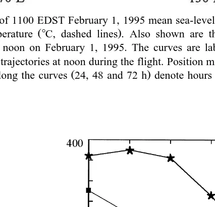
Fig. 1. Map of 1100 EDST February 1, 1995 mean sea-level isobars hPa, solid lines and average weekly sea
Ž .
surface temperature 8C, dashed lines . Also shown are the 72-h back trajectories for air that was W of Tasmania at noon on February 1, 1995. The curves are labelled 800, 900 and 1000 to denote the pressure levels of the trajectories at noon during the flight. Position marks are given for each 12 h along the trajectories.
Ž .
The labels along the curves 24, 48 and 72 h denote hours prior to noon February 1, 1995.
labels far W of Tasmania. After that, the air subsided under the influence of the large high-pressure system, and the wind speed was reduced. Twelve hours prior to the flight,
the mean boundary-layer air speed was 10 m sy1, but during the flight, the wind in the
Ž y1.
boundary layer was light 4–6.5 m s from W–NW. During the 72-h period, the air
close to the surface experienced an increase in sea surface temperature of as much as
118C. In the last 12 h, the change in sea surface temperature was quite modest, probably
only a fraction of a degree.
Fig. 3 is a NOAA-9 visual satellite image from 1007 h showing Tasmania and the Southern Ocean. The image shows numerous mesoscale cloud structures — closed cell convection — with typical horizontal scales of about 30 km. The cells are separated by subsidence lines, which contain thin cloud or clear air on much smaller scales. All observations in this paper will be presented in a coordinate system advecting towards the
SE at 4 m sy1. A distance scale has been added to Fig. 3. The F27 observations were
taken along this scale and it will be used as a reference throughout the paper. The 4 m sy1
advection speed was determined by iteration to ensure that cumulus clouds are
nearly vertical in the advecting coordinate system. The 4 m sy1 speed was also the mean
along-track wind speed near the surface. Using this advective coordinate system, observations taken at different times can be related to one another; this is important for studying vertical coherence and also for relating aircraft observations to positions on the satellite image.
A number of linear cloud features were observed both from above and below the cloud deck, some of these features being visible on the satellite image. One example is
Ž
the band apparent in the closed circulation beyond the NW end of the distance scale see
.
the small arrows in Fig. 3 . A number of cumulus bands were penetrated to the SE of this one during the flight; the first one was located in the closed cell circulation centred on the 10-km mark on the distance scale in Fig. 3.
The F27 entered the area at 1027 h that was 20 min after the satellite pass. Over the next 2.5 h, the stratiform decks and cumulus clouds persisted and developed. A second flight later in the afternoon showed that the pattern of stratus decks and cumulus continued throughout the day.
2.2. Terminology
Ž .
Albrecht et al. 1979 described a model of cumulus clouds in the marine boundary
Ž .
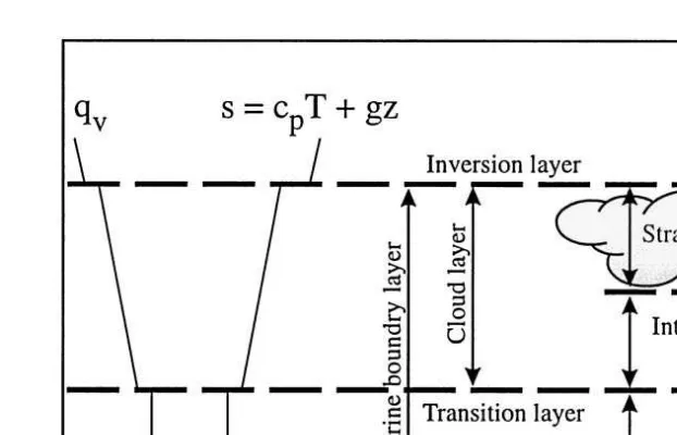
layer, and we will adopt a similar terminology see Fig. 4 . They examined a case in which there were positive heat and moisture fluxes from the sea surface. Close to the sea
Ž .
surface is a mixed-layer in which both water vapour mixing ratio qv and dry static
Ž .
energy s is assumed well mixed. The mixed-layer is assumed saturated at the top and capped by a small inversion, referred to as the transition layer. The top of the mixed-layer is also the base of cumulus clouds. These clouds define a cloud layer to the
Ž .
marine boundary-layer inversion see Fig. 4 . It is possible to have profiles of vapour mixing ratio and dry static energy such that the top of the cloud layer is saturated everywhere, i.e. an upper level stratus deck may exist. The subsaturated layer below the stratiform layer will be called the intermediate layer. The mixed-layer and cloud layer
Ž .
Fig. 4. Idealised thermodynamic profiles and the terminology of the marine boundary layer. The two idealised
Ž . Ž .
profiles show dry static energy s and water vapour mixing ratio q .v
profiles are convenient idealisations of actual boundary layers. In the present case, a more complex boundary layer structure will be documented.
2.3. Flight plan
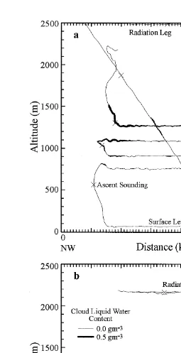
Fig. 5a and b shows the flight tracks for two stacks from the first flight on February 1 projected onto a vertical plane. A flight stack consists of horizontal legs of about 30–40 km length and a sounding from above cloud top to near sea surface. The stack commenced with a horizontal leg about 700 or 1000 m above cloud top for radiation
Ž .
measurements the radiation leg , followed by a turn and descent to 60 m above sea
Ž . Ž
level the descent sounding . Then, a horizontal leg was made at 60-m height the
. Ž .
surface leg , after which an ascent to 800 m was made the ascent sounding . This was
Ž
followed by four horizontal legs, which were partly or fully in cloud the four cloud
.
legs , the lowest three of which were through cumulus clouds at various times. The highest cloud leg was generally in solid cloud for 30–40 km, mostly in a stratus deck, but at times in the upper portions of the cumulus clouds penetrated into the stratus cloud. The track line in Fig. 5a and b has been made bold where cloud liquid water is
Ž .
present. The first stack Fig. 5a shows extensive cloud liquid water at the ends of the track, particularly in the NW end, which are associated with relatively deep cumulus clouds. The descent sounding in the middle goes through a shallow stratiform cloud deck, which is also penetrated by the aircraft in the upper of the four cloud legs. The
Ž .
Ž . Ž . Ž .
Wind hodographs were created from average wind direction and speed for each of the
horizontal legs, with the near surface wind slightly less than 4 m sy1 and from
W–WNW. The cloud legs have winds nearer NW and speeds of 4.5–6.5 m sy1, while
the radiation legs, 700–1000 m above the inversion, showed wind speeds increasing to 9
m sy1 with a northwesterly direction.
3. Observations from stack 1
3.1. Cloud top
The top of the marine boundary-layer cloud was monitored by forward and down-ward looking video cameras. The cloud top was visually quite uniform along the first radiation leg, but a band of cumulus was visible a few kilometers NW of the end of the
Ž .
flight track near 0 km on the distance scale; see Fig. 3 . This cumulus band was roughly perpendicular to the flight track and was estimated to be tens of kilometres long. The band was visible as several cumulus domes, each of which was estimated to overshoot the stratiform cloud top by no more than 100 m.
3.2. Vertical profiles
After completing the radiation leg above cloud, the aircraft made a descent almost to
Ž .
the sea surface towards SE see Fig. 5a . After a surface leg, the aircraft ascended to 700 m at the NW end of the stack. Profiles from these two soundings are shown in Fig. 6a–f.
Ž .
During the descent, the top of the solid stratiform cloud deck was at 862 hPa 1350 m ,
Ž .
and the less well-defined base at 892 hPa 1060 m . Some smaller fractus clouds were observed below the main stratiform base.
Ž .
Fig. 6a shows a profile of the virtual potential temperature uv , here defined as:
uvsu
Ž
1q0.61 qvyql.
Ž .
1where q and q are the vapour mixing ratio and the cloud liquid water mixing ratio,v l
respectively. Fig. 6b shows the vertical profile of q , and Fig. 6c shows the verticalv
Ž .
profiles of q from the King probe and of drizzle mixing ratio ql p from the 260X
probe. The profiles of uv and q have been made bold whenever the aircraft measuredv
solid cloud in a 1-s sample. This was done by requiring that all 64 samples within a
Ž
second contained cloud drops. The mixed-layer below 918 hPa, as measured during the
.
descent sounding is not entirely neutral in stability; the lowest part of the descent sounding below 300 m altitude reveals cooler air. After the completion of the descent sounding, the aircraft penetrated a shower and the cool air observed in the descent sounding may be caused by evaporation of precipitation from this shower.
The profile ofuv for the ascent sounding to 700 m, at the NW end of the flight track,
appears to show a slightly warmer and neutrally stratified mixed-layer. However, the
corresponding profiles of q from the two soundings are not at all well mixed. There isv
a decrease of almost 1 g kgy1 from the surface to the top of the mixed-layer, and
Ž . Ž . Ž .
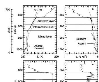
Fig. 6. Vertical profiles from stack 1 of a virtual potential temperature,uv; b vapour mixing ratio, q ; cv
Ž . Ž .
cloud and drizzle liquid water mixing ratio, q and q ; d relative humidity, RH; and e wind direction, Dir.l p
Ž . Ž . Ž .
The horizontal wind speed u and turbulent vertical velocity wrm s are shown with thin and bold lines in f . The wind direction and speed are given relative to the ground. The measurements are for the descent sounding unless otherwise noted. The first two boxes also show observations from the corresponding ascent sounding. Theuv and q lines have been made bold in solid cloud. A largev qdenotes values for the LCL. Dashed lines
Ž . Ž .
are predictions based on adiabatic ascent from the LCL Cu or stratiform cloud base Sr .
Ž .
Fig. 6a shows virtual moist adiabats from a lifting condensation level LCL
Ž .
determined from surface leg measurements to be described later and from the base of the stratiform deck; these are labelled ‘‘Cu’’ and ‘‘Sr’’ in Fig. 6a, respectively. The
pressure and temperature of the LCL are 945 hPa and 9.78C, and for the stratiform base,
they are 892 hPa and 6.58C. Notice that the LCL level is as much as 25 hPa below the
apparent top of the mixed-layer.
The observed profile of uv in the stratiform cloud deck appears to be stable with
regard to moist adiabatic processes. Other results, presented in Appendix A, suggest that the cloud deck is nearly neutrally stratified; the apparent cloud layer stability in Fig. 6a is likely the result of a slow response of the Rosemount temperature sensor housing,
Ž .
such as described by Rodi and Spyers-Duran 1971 . The implication is that the
too high during the descent sounding. We suspect that the real gradient of uv in the
Ž
stratiform cloud is, in fact, much closer to the gradient predicted by adiabatic ascent see
.
Appendix A .
The descent sounding thus shows four de-coupled layers below the marine boundary
Ž .
layer inversion: i the uv gradient is likely close to moist adiabatic in the stratiform
Ž .
cloud, ii it is very stable with regard to dry adiabatic motions in the intermediate layer
Ž . Ž .
below the stratiform cloud, iii it is nearly neutral in most of the mixed-layer and iv quite stable in the lowest 300 m above sea surface. The stable layer lowest to sea surface
Žthe cold pool is of limited horizontal extent..
Fig. 6c shows the observed values of cloud liquid water mixing ratio, and the corresponding values based on adiabatic ascent, from both the LCL-determined cloud base of the cumulus clouds and from the observed base of the stratiform clouds. The
stratiform cloud deck has strong vertical variations in q , and both entrainment andl
drizzle production may contribute to this variability. The stratiform cloud base is quite ill-defined due to the fractus clouds below, and it is therefore difficult to say to what extent the stratiform cloud has less water than the value based on adiabatic ascent. Drizzle, as measured by the 260X probe, constitutes a significant fraction of the total condensed water in the stratiform cloud, and drizzle from the stratiform cloud deck extends to below the top of the mixed-layer.
Ž .
Relative humidity Fig. 6d decreases from the stratiform cloud base towards the sea surface, although the value is always greater than 75% below the stratiform cloud.
Wind direction and speed are shown in Fig. 6e–f, with wind direction being generally westerly at low levels and changing to more northwesterly with height. Wind speed was in general greatest in the air above the inversion. In the stratiform cloud deck, the wind speed decreased substantially, before increasing closer to cloud base. Throughout the marine boundary layer, the wind speeds were quite small with values between 3 and 7 m
sy1. The high variability, in both wind direction and speed, is probably caused by
mesoscale circulations setup by the closed cell structure of the convection.
A measure of the turbulence intensity has been calculated by filtering the 64 samples
Ž .
per second vertical velocity w series from the descent sounding such that only
frequencies between 1 and 10 Hz remain. The resulting series was then used to calculate
a 1-Hz root-mean-square velocity, wrms. This series was subsequently smoothed with an
11-s running mean, and the result is shown in Fig. 6f. It can be seen that the turbulence intensity is highest in the middle of the stratiform cloud, that it is generally low in the mixed-layer, before again increasing as the aircraft enters the cold pool 300 m above the surface.
3.3. Mixed-layer properties
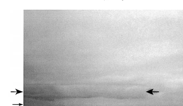
A surface leg towards NW was made after the completion of the descent sounding. A photo, taken at the 23-km mark on the surface leg looking NW, shows a very
Ž .
pronounced band of cumulus convection see large arrows in Fig. 7 . This cumulus feature will be referred to as Band 1. It is located at the 12–16-km mark on the distance
Ž .
scale Figs. 3 and 5a , i.e. in the turn, after the completion of the surface leg. Another
Ž .
Ž .
Fig. 7. Photo of cloud base from the first surface leg taken at the 23-km mark 1057 h looking towards NW.
Ž .
A band of cumulus convection can be seen below the stratiform deck band 1, large arrows ; this band is at the
Ž .
12–16-km mark on the distance scale. Further in the distance is the very long band of cumulus small arrows .
This is towards the region where the satellite image shows a cloud band NW of the
Ž .
flight area see small arrows in Fig. 3 .
Ž .
Measurements along the surface leg 60 m altitude show considerable variability in
Ž . Ž
thermodynamic parameters see Fig. 8a–e , for example, vapour mixing ratio q ; Fig.v
. y1
8a has variations of up to 1 g kg along the track. This is not surprising given the
Ž .
large vertical gradients in q observed during the descent sounding Fig. 6b . The virtualv
Ž .
potential temperature Fig. 8b shows a marked minimum in the SE end of the track. This is where Fig. 5a shows a cloud with high liquid water content immediately to the SE of the track; the cold pool is likely the result of evaporating precipitation from this cloud. The virtual temperature trace increases slowly towards the NW to reach a value
18C higher than in the centre of the cold pool. The descent sounding showed that this
Ž .
cold pool was less than 300 m deep. The pressure of the LCL pLC L shows variations
Ž .
within a 25-hPa range see Fig. 8c . The sea surface temperature, as measured from a
Ž .
downward looking infrared thermometer Barnes PRT-5, not shown , has values of 16.2"0.28C over the 40-km long surface leg. The sea surface temperature is in general
1.38C higher than the air temperature immediately above the sea surface, which implies
a positive heat flux from the sea surface to the air. The cold pool is even colder than the rest of the mixed-layer and hence much colder than the sea surface. Therefore, the cold pool must have been created by evaporation of falling precipitation.
Ž .
The along-track horizontal wind component ut in the advecting coordinate system is
shown in Fig. 8d. The flight track was nearly perpendicular to the cumulus band in the NW end of the flight track, and the along-track wind shows significant variations. In the
Ž . Ž .
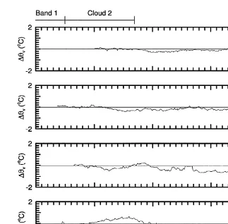
Fig. 8. Surface leg along-track variation of a vapour mixing ratio, q ; b virtual potential temperature,v uv;
Ž .c LCL pressure, pLC L; d along-track wind speed, u ; and e along-track convergence, C , for stack 1.Ž . t Ž . t
NW, and the centre of the track shows no net along-track wind component relative to the advecting coordinate system. The along-track wind is used to calculate the along-track
Ž .
convergence Cts yd utrd x; Fig. 8e , where x is the distance along the track. This
Ž .
series has been filtered with a 31-s 2.5 km running mean, and the first and last segments of the series have been omitted. The along-track air flow is divergent at the far
Ž . Ž .
NW end of the track NW of 19 km , and in the subsequent turn not shown , there are traces of drizzle. Between 19 and 26 km, there is a strong, and near solid, region of along-track convergence, and the region between 26 and 40 km is devoid of systematic along-track convergence or divergence. Further to the SE, there is primarily light
Ž
along-track convergence. The region with the lowest virtual potential temperature 54
.
km and beyond; see Fig. 8b is divergent in the along-track direction. Later, a cumulus band was observed to grow over the 19–26 km along-track convergence zone, and the
Ž .
thermodynamic parameters for this segment have been used to calculate the LCL q
shown in Fig. 6a and b.
3.4. The cloud legs
Ž .
Ž .
from the descent sounding 918 hPa; Fig. 6a . Analysis, to be presented later, shows that the mixed-layer height varies along the track. The lowest cloud leg appears to be partially in the mixed-layer and partially above the top of the mixed-layer.
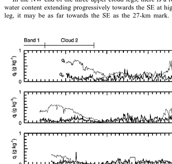
Observations of cloud and drizzle water mixing ratio, for the four cloud legs and the surface leg, are shown in Fig. 9a–e. The surface leg is virtually free from drizzle, but
Ž .
small traces are apparent in the far SE end of the track 56–57 km . Cloud liquid water
Ž .
in the lowest cloud leg Fig. 9d, thin line is only apparent NW of the 15-km mark; this
Ž .
is part of the cumulus band visible in Fig. 7 Band 1 .
In the NW end of the three upper cloud legs, there is a region with high cloud liquid water content extending progressively towards the SE at high altitudes. In the top cloud leg, it may be as far towards the SE as the 27-km mark. This indicates that a strong
Ž .
Fig. 9. Cloud and drizzle liquid water mixing ratio q and q , respectively for the four cloud legs and thel p
surface leg in stack 1. The top box shows the values for the highest flight leg, the bottom box for the surface
Ž .
leg. Cloud liquid water is measured using the King probe thin line and drizzle water is from the 260X probe
Žbold line , class 5 and larger drops; i.e. r. )22.5 nominally. A brief data system error is apparent in theŽ Ž ..
Ž .
cumulus cloud grew over the main surface along-track convergence 19–26 km while the F27 executed the three upper cloud legs. This cloud is directly on the SE side of cumulus Band 1. Due to low visibility, evident in video recordings, it could not be determined if this cumulus feature was band-shaped; it will therefore be called cumulus Cloud 2. This cumulus is the first of the cloud features that is not readily identifiable in
Ž .
the satellite image Fig. 3 obtained an hour earlier.
A solid stratiform deck is also apparent SE of the 30-km mark in the cloud top leg and to a lesser extent in the cloud leg below. Both of these cloud legs also show what appears to be a small cumulus cloud around the 45-km mark.
The drizzle mixing ratio is very high, particularly in and below the stratiform cloud region. In the highest cloud leg, close to half of the condensed water in the stratiform cloud is contained in drizzle-sized drops. The cloud liquid water is much higher than the drizzle water content in the solid cumulus clouds, the young age of the cumulus clouds being a possible explanation for this difference. Drizzle from the stratiform cloud is
Ž .
apparent even in the lowest cloud leg 28–50 km; Fig. 9d .
The buoyancy field is of considerable interest for this cumulus and stratocumulus system, though, due to horizontal variability, it is difficult to define a representative sounding for such a complicated system. Table 1 shows a simplified sounding that is based on selected measurements from stack 2. This sounding is solely used as a simple reference, so that buoyancy can be calculated relative to it. Fig. 10 shows the virtual
Ž .
temperature excess Duvsuvyuvs p , where uv is the virtual potential temperature
Ž .
from the aircraft during the flight legs, and uvs p is the value for the reference
Ž .
sounding at pressure p see Table 1 .
Ž .
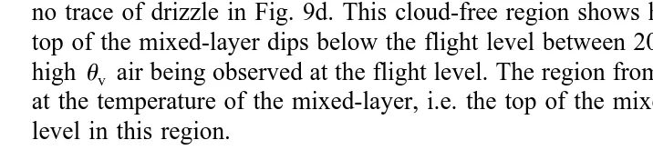
In the lowest cloud leg Fig. 10d , a cold air region is apparent from 30 to 52 km.
This region is almost identical to the region with light drizzle shown in Fig. 9d. TheDuv
field shows a pronounced maximum between 20 and 30 km. This coincides with little or
no trace of drizzle in Fig. 9d. This cloud-free region shows high uv suggesting that the
top of the mixed-layer dips below the flight level between 20 and 30 km; this results in
highuv air being observed at the flight level. The region from 30 to 52 km is essentially
at the temperature of the mixed-layer, i.e. the top of the mixed-layer is above the flight level in this region.
Table 1
Simplified reference sounding
Values from below 918 hPa are loosely based on the stack 2 ascent sounding; values from above 918 hPa are from the stack 2 descent sounding. Note that no transition layer jump is included in this table.
Ž .
Fig. 10. Buoyancy, expressed as Duv from the reference sounding Table 1 , for the four cloud legs and
Ž Ž ..
surface leg from stack 1. A brief data system error is apparent in the centre of c .
The virtual temperature patterns in the top two cloud legs are quite similar. There are maxima at the two ends of the flight legs and a broad minimum at the centre. The region
Ž .
of maximum cloud liquid water at the NW end Fig. 9a and b coincides with one of the most buoyant regions in Fig. 10a and b.
Ž . Ž .
The vertical wind speed w, bold line and along-track wind speed u , thin line aret
shown for the same five legs in Fig. 11a–e. The surface leg has quite modest and fairly small-scale vertical velocities. The strong along-track convergence region in the surface leg between 19 and 26 km is not readily apparent in the vertical velocity at the same level. This may be because the surface leg is made as low as 60 m above the sea surface;
y4 y1Ž .
a convergence of 5=10 s see Fig. 8e between 0 and 60 m results in an updraft of
just 0.03 m sy1 at 60 m altitude. If the same convergence is present over the depth
Ž .
between surface and the LCL 0–600 m , then the resulting mean updraft at the LCL in
the 19–26 km region would be 0.3 m sy1. The along-track convergence pattern is thus
Ž . Ž .
Fig. 11. Vertical velocity w, bold line and along-track wind speed u , thin line for the four cloud legs andt
Ž Ž ..
surface leg in stack 1. A brief data system error is apparent in the centre of c .
and downdrafts in the cloud legs are found in the NW end of the track and appear to be related to cumulus Band 1 and cumulus Cloud 2.
Ž .
The along-track wind component ut in the advecting coordinate system is shown in
Fig. 11 with the thin lines. The lowest two cloud legs show very low values of u NWt
of the 25–27-km mark. It is not apparent why the strong cloud layer gradients in u aret
located in this position; the location does not coincide with the cumulus edge or the stratiform drizzle region.
4. Observations from stack 2
At the completion of stack 1, there was a mature cumulus band in the far NW end of
Ž . Ž .
the far SE end of the flight track. Cloud 2 matured during the time it took to fly stack 2, and the cumulus cloud in the far SE is not apparent at later times. During the time stack
Ž . Ž
2 was flown, a new cumulus band Band 3 developed in the centre of the stack Fig.
.
5b where previously only a stratiform cloud existed. The manner in which this band appeared to be forced by the maturation of Cloud 2 will now be described.
4.1. Vertical profiles
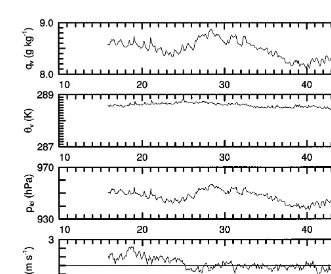
Fig. 12a–f shows vertical profiles of thermodynamic, microphysical, and wind parameters for the descent sounding, which began in the SE end of the stack and
Ž .
finished near the surface in the far NW end see Fig. 5b . Some of the profiles also show values for the ascent sounding to 800 m, which was made in the SE end of the stack.
Ž .
The virtual potential temperature profile Fig. 12a shows an inversion of about 2.58C
at 848 hPa, and a stratiform cloud layer between 848 and 880 hPa. Below this is a layer
Ž .
with, on average, stable stratification, but with strong variability 880–925 hPa . Video recordings show that the aircraft, at 920 hPa, skimmed the top of a small cumulus band,
which later grew to dominate the cloud field. The small decrease in uv at 920 hPa may
well be due to mixing between this cumulus band and clear air. At 928–926 hPa, there
is a small transition layer, marking the top of the mixed-layer found in the descent sounding.
The descent sounding shows this ‘‘mixed-layer’’ as having an almost neutral stratification in the upper portion. Lower down, the virtual potential temperature
decreases to about 1–1.58C less than at higher levels. This cold pool in the NW end of
the descent sounding may have resulted from the evaporation of 0.4–0.6 g kgy1 of
precipitation in the mixed-layer. Sea surface pressure is calculated to be 1012 hPa. After reaching 60 m altitude, the aircraft turned around, made a 40-km surface leg, and ascended to 800 m in the SE end of the flight stack. Fig. 12a also shows the virtual temperature from this ascent. It can be seen that a neutrally stratified mixed-layer
Ž .
extends all the way to 918 hPa 800 m at this end of the stack, i.e. at this stage, the
precipitation-cooled air is confined to the NW end of the stack. Theuv profiles for the
descent and ascent soundings match one another closely in the narrow range of 930–940
Ž .
hPa, but the ascent sounding is neutrally stratified to a higher level 918 hPa .
Ž .
Fig. 12a also shows with a boldq the pressure and virtual temperature for a LCL
determined from surface leg measurements; the pressure and temperature at the LCL are
939 hPa and 9.28C, respectively. The uv profile for a parcel ascending adiabatically
from this LCL is shown with a dashed curve, labelled Cu in Fig. 12a. Air ascending adiabatically from the LCL has an alternating small positive or negative buoyancy in the first 40 hPa above the LCL. Higher up, the buoyancy is systematically positive for an adiabatically ascending parcel, but the excess virtual potential temperature is always less
than 0.58C. The instability in the cloud layer is quite modest, with a convective available
Ž . 2 y2
potential energy CAPE of about 3 m s .
The figure also shows the virtual potential temperature of a parcel ascending moist adiabatically from the base of the stratiform cloud deck, labelled Sr. The virtual potential temperature gradient in the stratiform cloud is shown to be more stable than a moist adiabat. As for stack 1, we believe that this apparent stability in the stratiform deck is largely an instrumental artifact caused by the slow time response of the
Ž .
Rosemount temperature sensor housing see Appendix A .
Fig. 12b shows the vapour mixing ratio, q , for both the descent sounding and for thev
800-m ascent made after the completion of the surface leg. The ‘‘mixed-layer’’ is well
Ž . Ž
mixed in uv Fig. 12a away from the cold pool, but it is not well mixed in qv Fig.
.
12b . There is both a strong mean vertical gradient in q and local variability, the latterv
presumably due to the localised nature of evaporating drizzle and to individual thermals rising from the sea surface. The vapour mixing ratio in the descent sounding is, in general, lower than that in the ascent sounding. This is consistent with evaporation of precipitation in the cold pool part of the descent sounding. The cooling of air due to evaporation may lead to downdrafts and thus bring down air that is comparatively low in
Ž
vapour mixing ratio. The vapour mixing ratio of the LCL determined from the surface
. y1 Ž
leg is about 1 g kg higher than the mixed-layer air at the same level see the boldq
.
in Fig. 12b .
The vertical profile of cloud liquid water mixing ratio determined from the King probe is shown in Fig. 12c. Also shown in this figure is the drizzle water mixing ratio
from the PMS 260X probe for drops larger than 23mm radius. Drizzle observed during
levels from the cloud top to about 30 hPa below the stratiform cloud base. Some drizzle is also observed in the lower part of the descent sounding, both in the top part of the mixed-layer and in the cold pool. The maximum drizzle water mixing ratio is about half the maximum cloud water mixing ratio, though at different altitudes. The figure also shows the calculated liquid water mixing values assuming moist adiabatic ascent from
Ž . Ž
both the LCL curve labelled Cu and for the base of the stratiform cloud curve labelled
.
Sr . The reduction in cloud liquid water from the adiabatic values in the stratiform cloud could be due to drizzle and entrainment, but also to uncertainty related to the determina-tion of the stratiform cloud base.
The relative humidity in clear air has important effects on the evaporation of drizzle drops below the cloud and on entrainment. Fig. 12d shows the vertical profile of relative humidity for the descent sounding. The air between the LCL and the stratiform cloud is very moist with relative humidity larger than 85%; this is partly caused by evaporation of drizzle. The air in the first 50 m in and above the marine boundary-layer inversion is also comparatively moist, with a relative humidity of 75%. A further 50 m higher, the relative humidity decreases to about 50%. Wind direction and speed for the descent sounding are shown in Fig. 12e–f; as was the case for stack 1, the winds are light and
Ž . Ž .
Fig. 13. Surface leg along-track variation of a vapour mixing ratio, q ; b virtual potential temperature,v uv;
Ž .c LCL pressure, pLC L; d along-track wind speed, u ; and e along-track convergence, C . The measure-Ž . t Ž . t
Ž .
Ž .
variable. The turbulence level wrms; Fig. 12f is again high in the centre of the
stratiform cloud, somewhat lower below the stratiform cloud, low in the upper part of the mixed-layer, and high further down as the aircraft enters the cold pool in the lower mixed-layer.
4.2. Mixed-layer
Ž .
Measurements of thermodynamic parameters from the surface leg 60-m altitude show considerable variability over the 32-km flight distance from NW towards SE. Three segments can be identified from the thermodynamic and dynamic parameters shown in Fig. 13a–e.
Ž
The surface leg commenced in a region of light, intermittent drizzle segment A,
.
18–28 km in Fig. 13a .
Ž .
This segment shows the highest values of vapour mixing ratio q , the highest LCLv
Ž .
pressure i.e. LCL is closest to the sea surface , and the lowest virtual potential
Ž .
temperature uv . The lowuv implies that this air is unlikely to ascend, and so defines
the cold pool.
Ž .
The next segment B, 28–34 km in Fig. 13a shows the lowest values of q but av
considerably higheruv. The air can readily ascend if forced, but the dryness of the air
ensures that the LCL pressure is very low; i.e. the air in segment B must be forced high up before condensation begins.
Ž .
Further towards the SE is segment C SE of the 34-km mark in Fig. 13 , which is characterised by warmer and slightly dryer air than segment A, but which is more moist than segment B. Segment C has a LCL that is intermediate between those of segments A
Ž .
Fig. 14. Photo of cloud base from the second surface leg 1207 h at the 26-km mark. Note the band of shallow
Ž .
and B. Segment C is by far the most likely source for air entering the cumulus cloud bases, as the air is both warm and moist.
Ž .
The LCL pressure, pLC L, varies by 30 hPa along the flight track see Fig. 13c . The
cloud base, calculated from the average LCL parameters for segment C, is 942 hPa and
Ž .
9.3. The altitude of the LCL is 615 m. The virtual moist adiabat ‘‘Cu’’ in Fig. 12a is based on the LCL determined from segment C.
Ž .
The along-track horizontal wind component in the advecting coordinate system ut is
shown in Fig. 13d. The flight track was nearly at right angles to the cumulus band. In
region A, u increases fromy1 to 3 m sy1 before settling back to 1 m sy1 in the SE
t
end of region A. This pattern is consistent with a downdraft spreading out in region A.
In region B, the value of u decreases gradually towards the SE, and a few kilometrest
into region C, it takes on a fairly uniform value ofy1 toy2 m sy1.
Fig. 13e shows the along-track convergence, C . NW of the 23-km mark, there ist
strong along-track divergence. This divergence is located immediately below the centre
Ž .
Fig. 15. Cloud and drizzle liquid water mixing ratio q and q , respectively for the four cloud legs andl p
of Cloud 2 as determined from Fig. 9. From 23 to 35 km, there is a fairly persistent along-track convergence pattern, and further towards the SE, there is no net along-track convergence or divergence. This pattern is consistent with a downdraft in region A spreading out and forcing the lowest part of the mixed-layer for a distance of 15 km further to the SE. Note how the along-track convergence extends into the far NW part of region C, which the thermodynamic analysis suggests as the source of air most likely to ascend into cumulus clouds.
Ž .
The sea-surface temperature as determined from the Barnes PRT-5 not shown has
values of 16.0"0.28C along the surface leg. The air immediately above the surface is,
on average, 1.18C colder than the sea surface.
Ž .
A photo looking towards SE was taken at the 26-km mark 1207 h during the surface
Ž .
leg see Fig. 14 , and showed two bands of cumulus clouds visible below the stratiform cloud deck. The nearest band is visible as a string of very shallow cumulus, estimated at no more than 100–200 m deep; video recordings show that these are located at the
Ž .
33-km mark. This shallow cumulus band was also observed during the descent sounding at the same location 7 min earlier. We will now show how this cumulus line developed and ended up dominating the cloud field.
4.3. The cloud legs
Cloud and drizzle liquid water mixing ratio, from the surface leg and four cloud legs, are shown in Fig. 15. A very pronounced cumulus cloud is evident from the 34–40-km region at low levels and in a somewhat wider region at the highest level. Video recordings from the lowest cloud leg show that it is a cumulus band located where the very shallow band of cumuli were observed in Fig. 14. This band has been described by
Ž .
Boers et al. 1997 and will be referred to here as Band 3.
The drizzle water contents in the four cloud legs are very large, in some regions even exceeding the cloud liquid water content. It is noted that the drizzle water content is very
Ž . Ž .
Fig. 17. Vertical velocity w, bold line and along-track wind speed u , thin line for the surface leg and fourt
Ž .
low in the new cumulus band Band 3 and high in the mature cumulus cloud in the NW
Ž .
end Cloud 2 .
The virtual temperature difference between observations and the reference sounding
ŽTable 1 , expressed as. Duv, along the surface leg and the four cloud legs is shown in
Fig. 16. For the four cloud legs, the figure shows thatDuv is high at the two ends of the
track and relatively low in the centre. The new cumulus band is positively buoyant
Ž .
relative to its immediate environment in the two lower cloud legs Fig. 16c and d . The lowest cloud leg is close to the top of the mixed-layer. As for stack 1, there is a possibility that a small segment of this leg is above the top of the mixed-layer, e.g. the relatively warm segment from 25 to 29 km.
Ž .
The vertical velocity for stack 2 is shown in Fig. 17. The new cumulus band Band 3
Ž .
dominates the velocity variations in the lower three cloud legs Fig. 17b–d . In the top cloud leg, the cumulus shows very modest updrafts and downdrafts, which are indistin-guishable from the remainder of the top cloud leg.
Ž .
The along-track wind u , thin line in Fig. 17 shows Band 3 to be in a region oft
Ž .
broad along-track divergence high u on the SE side, low u on the NW side ; this ist t
particularly clear in the lower two cloud legs. The two upper flight legs show along-track divergence within Band 3.
5. Discussion
In this section, we discuss the interaction between the three ‘‘generations’’ of cumulus clouds. The existence of the cold pools in the mixed-layer is shown to be essential to the cloud organisation. Therefore, we will use a simple model to compare the mixed-layer development inside and outside a cold pool.
5.1. ConÕectiÕe organisation
The cloud fields developed considerably over the 2.5 h of flying time. At least two, possibly three, cumulus bands were observed in various stages of inception, new growth, maturation, and dissipation.
The existence of cumulus bands is based on visual observations. The band shape could only be determined from the cloud appearance during the surface and the lowest cloud legs. At higher altitudes, the same cloud formations were observed, but they were obscured by falling drizzle or they were entirely embedded in the stratiform cloud. Photographs from the flight legs above the boundary layer show some linear features but the orientation and length cannot be determined.
bands, there may be cellular structure along the bands. This is particularly clear in Fig. 14.
Cumulus Band 1 had a width of 2–3 km as measured close to the NE end of the band. Band 3 was penetrated closer to its centre and had a width of 5 km at low levels. It is uncertain if Cloud 2 was band-shaped. This cloud grew rapidly and was only observed during the three upper cloud legs where visibility was limited.
The bands appeared to be oriented in a SSW–NNE direction, which is roughly
Ž .
perpendicular to the near-surface wind W–NW . The bands were not penetrated strictly
Ž .
at right angles and their apparent width 2–3 and 5 km, respectively could be
Ž .
overestimates. The closed cell circulation evident in the satellite image Fig. 3 suggests that the bands were of limited length. The ratio of length-to-width of a new band appears to be about 3:1. It would be unlikely that the bands were as long as the scale of the closed cells apparent in the satellite image, since this would imply abrupt transitions at the end of the cumulus bands. It is unclear if cumulus bands are a common feature of closed cell circulation, and, if they are, whether the orientation is commonly perpendicu-lar to the low-level wind. As a cold air downdraft spreads out, it may have a tendency to form an arc of increasing radius. The new convection may form where a spreading cold pool ‘‘collides’’ with a moist and warm part of the mixed-layer. This could in principle lead to arc-shaped or near-linear cumulus bands. If this mechanism is taking place, then the orientation of the bands would not depend on the mean wind direction or mean vertical shear. The satellite image shows reflectivity maxima that in some cases are linear, but the lines appear to have a variety of orientations. The aircraft observations show cumulus clouds with high droplet concentrations, high albedo, and low effective
Ž ` Ž . 3 4 ` Ž . 2 .
radius res H0n r r d r rH0n r r d r, Hansen and Travis, 1974 . This may be a
useful signature for satellite determinations of the linearity of cumulus bands embedded in stratocumulus.
Ž .
Wang and Lenschow 1995 flew through a series of cumulus clouds that grew into a stratocumulus deck. Their stacked flight legs were roughly perpendicular to the mean
surface wind; i.e. turned 908relative to our measurements. They found that the cumulus
clouds at higher levels were visible for 36 km along the track. They used an upwards pointing lidar to determine cloud base, and these measurements show several cumulus cells along the track. However, no photographs of the clouds were shown and band structure was not discussed.
The closed cell structure apparent in the satellite image pertains to the cloud layer. The cell structure may be different in the mixed-layer due to the presence of up to four
Ž .
decoupled layers within the marine boundary layer see Sections 3.2 and 4.2 . The closed cell circulation appears to be sustained by the drizzle formation, the evaporation in the mixed-layer, and the ensuing forcing from spreading of evaporatively cooled downdrafts. It is therefore likely to be a cloud type more typical of clean air where
Ž
precipitation by coalescence processes are more likely. The air trajectory analysis Fig.
.
1 shows no continental influence in the 72 h prior to the flight. No sample with adiabatic liquid water content was observed from the aircraft in the cumulus, but an
Ž .
entrainment analysis Part II shows that cloud droplet concentration immediately above
cloud base in the new and solid cumulus bands must be in the range 155–235=106
kgy1. This droplet concentration is consistent with observations of CCN concentrations
Ž .
All of the aircraft observations are projected onto a coordinate system advecting at 4
m sy1 towards SE. This was found by trial and error to give the best vertical coherence
of cumulus clouds. The 4 m sy1 is also the average along-track wind speed in the
surface flight legs, and closer to the inversion, the along-track wind speed increased to
4.5–6.5 m sy1. The advecting coordinate system is not perfect; however, it is a
reasonable and necessary way of relating observations taken at different locations and times to one another.
From the aircraft wind measurements, it is not possible to calculate the complete horizontal convergence and divergence. Instead we use the aircraft wind measurements to calculate the along-track convergence and divergence components. For a boundary layer dominated by near-linear cumulus convection, this simplification yields a good
agreement between the variations in along-track convergencerdivergence components
and the cloud development aloft.
5.2. Synthesis of cloud eÕolution
The schematic evolution of the boundary layer is detailed in Fig. 18a–d. Each of these shows the flight tracks for a specific time period, roughly corresponding to half the time it took to execute a flight stack. As before, the flight track line is made bolder where cloud liquid water is observed. The figure also shows the outline of the cold pools
observed during each of the two stacks and of the along-track convergencerdivergence
field during the surface legs. The degree of cooling in the cold pools is shown with a cold front signature where the cold pool became apparent, and also with contours of
reduction inuv compared to other air at the same level. Arrows show where the highest
updrafts and downdrafts were observed; the size of the arrows is roughly proportional to
Ž .
the updraft speed. The top of the mixed-layer transition layer is shown with a bold dashed line. Above cloud top, the variation in short-wave albedo is shown. Some of the figures also show the variation of the effective radius as measured during the highest cloud leg. Drizzle mixing ratio is shown with shading. Some extrapolation from the flight tracks has been made, given that drizzle normally originates from a higher level and falls to a lower level, relative to the observation point.
Fig. 18a shows cumulus Band 1 in the NW end while apparently still in an early stage of development. The aircraft flew in the NE end of this band and the observations showed very little drizzle below the band. There is nevertheless a distinct along-track divergence and convergence pattern SE of Band 1 in the surface flight leg. It is possible that this is caused by precipitation falling from parts of Band 1 further to the SW. The cold pool and low-level circulations in the SE end of the surface flight leg are caused by precipitation from the mature cumulus above.
Ž .
A strong updraft is observed in Band 1 Fig. 18a . The mixed-layer top is lowest in
Ž .
the drizzle free region 15–28 km; Fig. 18a , whereas the mixed-layer top is much
Ž .
Ž .
The cloud top was below a height of 1400 m during the descent sounding Fig. 18a . It may have been higher above the cumuli, but this cannot be substantiated by measurements. The cloud albedo is low near the 20-km mark along the cloud top where a downward looking Barnes PRT-5 remote temperature sensor measured a very high cloud-top temperature. This feature may be a subsidence line between closed cell stratocumulus. The albedo is high over cumulus Band 1 and over the stratiform cloud closest to the cumulus to the SE.
Ž .
Fig. 18b shows that a substantial cumulus Cloud 2 grew up on the SE side of Band 1. This cloud formed over the along-track convergence region observed during the surface leg 20 min earlier. The proximity of this region to the along-track divergence region, observed further to the NW, suggests that Cloud 2 was forced by outflow created by evaporatively cooled air below Band 1, not from the cold pool much further to the SE. The new Cloud 2 was not observed during cloud leg 1 but was apparent as a solid cumulus when penetrated during cloud leg 2. The cloud subsequently ascended and spread to form a massive region with high liquid water content in the NW end of the track. At low levels, Band 1 and Cloud 2 were separated; at high levels, the distinction between them was not apparent. The inversion altitude had increased from 1400 to 1500 m when the aircraft finished flight stack 1. A small isolated cumulus was apparent during the two upper cloud legs near the 45-km mark. The difference between cumulus and stratiform cloud was very apparent in the albedo measurements.
At the beginning of stack 2, the stratiform cloud top height was also at 1500 m. Fig. 18c shows the descent through the stratiform cloud into the extensive drizzle below and through the tops of a band of small cumuli at the 35-km mark. Further to the NW, the aircraft flew into the cold pool generated by extensive evaporation of drizzle falling from Band 1 and Cloud 2. The cold pool setup divergence in the along-track direction, and an extensive region of along-track convergence occurred ahead of it, even further out than the limit of the cold pool. The band of small cumuli at 35 km was at the edge of the along-track convergence zone, and above a region of warm and moist air observed at the surface.
Fig. 18d shows that cumulus Band 3 subsequently grew and dominated the upwards motion in the area. During the previous surface leg, it was only visible as shallow cumulus humilis. During the first cloud leg, it was very fragmented at the penetration level, although some of the cloud elements may have reached the stratiform cloud. During cloud legs 2, 3, and 4, it was solid, indicating that strong growth took place after the aircraft had penetrated the cloud in the lowest cloud leg. The older convection in Cloud 2 was almost in the mature to dissipating stages at this point. The drizzle flux in
the lowest cloud leg below Cloud 2 was 0.4 mm hy1, but the cloud base was now raised
to a level between cloud leg 1 and 2. The strong drizzle flux from Cloud 2 suggests that the cold pool below continued to develop in the 20 min after the cold pool was first
Fig. 18. Schematic development of the marine boundary layer during the 2.5-h observation period. The flight track is thicker where cloud liquid water occurs. The shading is approximately proportional to drizzle water mixing ratio. The bold dashed line shows the top of the mixed-layer. The divergence and convergence labels
Ž .
refer only to the along-track component of the wind. Relative values of albedo and effective droplet radius re
Ž .
observed during the descent sounding of stack 2. The outline of the cold pool shown in Fig. 18d is shown as observed 15–20 min earlier than cloud leg 1. It is highly likely that the cold air pool has spread out during this time towards SE and that it forced the strong growth of cumulus Band 3.
With time, one would assume that Band 3 would spread out, and thus be the latest of a series of cumulus that provide moisture for the preservation of the stratiform shield. During the 2.5 h of observations, the boundary layer grew from 1350 to 1500 m, yet the stratiform cloud was still only about 300 m deep. This depth may be limited by both entrainment and drizzle formation. If the stratiform cloud deck was much deeper, then the drizzle formation would be even stronger. This would deplete liquid water and result in a thinner cloud deck.
The time evolution depicted in Fig. 18a–d shows an apparently persistent develop-ment of a convective system: cumulus bands form, precipitate, decay, and force new cumulus ahead of them. The convective system moves faster than the ambient wind, leaving processed cloud elements behind. This is a remarkable similarity to squall line systems in the free atmosphere, yet the present cumulus clouds are only 900 m deep in a 1500-m deep marine boundary layer. The observations show that clouds behaving as ‘‘deep convection’’ may occur in the boundary layer: evaporation of precipitation drives mesoscale circulations, which forces new convective elements. The video recordings and photographs show that some of these are band-shaped; for lack of a better term, we will call them boundary-layer squall lines. These bands may have lengths of at least 10 km and occur within cloud fields that the satellite image reveals as closed cell circulations. The present boundary-layer squall line system is different in a number of ways from the deep convection types. Firstly, the energetics are vastly different. The CAPE in these
clouds is only 13 and 3 m2 sy2, as determined from the descent soundings of stacks 1
and 2. Deep convection squall lines may be two orders of magnitude more energetic. Secondly, the aspect ratio is high in the present marine boundary layer: the cloud bands measured at low levels are typically 3–5 km wide in a cloud layer of only 900-m depth; i.e. an aspect ratio of about 3:1 to 6:1. Thirdly, the convection appears to move faster
Ž .
through the air than predicted by the theoretical study of Moncrieff 1981 . For a propagating system, Moncrieff predicts that the system speed through the air should be
2
'
in excess of the ambient wind speed by 0.32 CAPE . For an average CAPE of 8 m
sy2
, Moncrieff’s relationship predicts a 1 m sy1
speed relative to the surrounding air.
Ž
The observations shown here using positions from the lowest penetration of Bands 1
. y1
and 3 indicate a speed of 4.5 m s relative to the surrounding air.
Ž .
In a recent paper, Wyant et al. 1997 use a two-dimensional eddy-resolving model to simulate the marine boundary-layer development as air is moving SW in the Pacific Ocean towards the equator. Their simulation shows the cloud development from a solid low level stratus deck to isolated and deeper cumuli closer to the equator over a 10-day period. In the middle of their run, they show a 1250-m deep boundary layer with a combination of cumulus and upper level stratiform cloud. Wyant et al. use a 4-km wide domain for their main model, resulting in one or two cumulus cells; for a 12-km wide domain, three to four cumulus cells were found.
ob-served in the SOCEX case study were nearly a factor of 10 larger than in Wyant et al.
Ž1997 . This applies to both the cumulus band width SOCEX 3–5 km; Wyant et al. 0.5. Ž
. Ž .
km and to the distance between cumuli SOCEX 30–50 km, Wyant et al. -4 km .
This is apparent from both the aircraft observations and from the satellite image. The
drizzle rate near the top of the mixed-layer is 5 mm dayy1 as averaged over cloud leg 1
in stack 2. Wyant et al. show average drizzle rates for boundary layers of comparable depths that are only a few tenths of a millimeter per day. Our observations are only snapshots, and their representativeness is therefore somewhat uncertain, but the differ-ences between our study and the one of Wyant et al. are nevertheless substantial.
5.3. Mixed-layer and drizzle from cumulus
Ž
Classical marine boundary-layer models with cumulus convection e.g. Albrecht et
.
al., 1979 assume a mixed-layer where the top coincides with the LCL. The mixed-layer is assumed well mixed in terms of both energy and vapour mixing ratio. In the present Southern Ocean case, it is also convenient to consider a ‘‘mixed-layer’’ up to the LCL;
however, this mixed-layer is at best only well mixed in terms of uv, not q . Thev
localised occurrence of evaporating drizzle in the mixed-layer generates cold air masses,
which in turn drive mesoscale circulations. EÕaporatiÕe cooling is the significant effect
that separates the present mixed-layer from classical theory. Locally, where cold pools occur, the ‘‘mixed-layer’’ is stable; in other parts, the mixed-layer is unstable and allows for cumulus mass fluxes out through the top of the mixed-layer.
In a classical cumulus-topped mixed-layer model, there is a small inversion or stable
Ž .
layer at the top of the sub-cloud mixed-layer; Albrecht et al. 1979 called this the transition layer. Positive buoyancy fluxes from the sea surface may drive entrainment fluxes down into the mixed-layer from above this transition layer. When strong drizzle from the cumuli is present, the picture may be considerably more complicated. The observed mixed-layer, outside the cumulus-generated cold pools, has a nearly constant
Ž .
uv, but a marked decrease in qv with height Figs. 6b and 12b . The figures show an
average decrease in q of 0.7–1.0 g kgy1 over 800 m. Some decrease in q with height
v v
in the mixed-layer is common due to the primary source of moisture being the sea surface. Another observation is that the LCL, as calculated from the surface leg
Ž .
observations, is about 20–25 hPa below the top of the mixed-layer Figs. 6a and 12a . The LCL varies along the surface legs; the LCL values chosen here are for segments
that are both high in uv and q , as these are most likely to create the new cumulusv
clouds.
The cold pools, created by evaporating precipitation in the mixed-layer, are about 18C
colder than the remainder of the mixed-layer. The precipitation flux through the top of
the mixed-layer, required to cool the mixed-layer by 18C, will now be calculated. The
mass of an 825-m deep column of air is approximately 900 kg my2. To increase the
vapour mixing ratio by 0.4 g kgy1 requires a water amount of 0.36 kg my2 or 0.36 mm
of rain. The cooling of 18C can thus result from evaporation of a 1-mm hy1 drizzle
shower in 20 min.
parameterisa-tion of surface fluxes, and a simple entrainment assumpparameterisa-tion at the top of the cold pool based on buoyancy flux arguments. We assume a cold pool that is initially 100 m deep
and created by evaporating precipitation. It has an increase in mixing ratio of 0.4 g kgy1
relative to the surrounding mixed-layer, and consistent with this increase in q , it isv
Ž .
initially 18C colder than the mixed-layer see Fig. 19a and b . The sea surface is
assumed to be 28C warmer than the air in the cold pool at the start of the model
calculation, and surface fluxes are driven by a 4 m sy1 wind speed. The choice of these
parameters is based on the aircraft observations.
Ž .
Over 3.5 h, the cold pool grows in depth from 100 to 150 m see Fig. 19 . It also
increases the vapour mixing ratio by almost 1 g kgy1, such that it is far more moist than
the remainder of the mixed-layer. It is thus possible, that cold pools can exist for hours before the temperature recovers to values typical of the rest of the mixed-layer, and during this time, they may force air motions in the mixed-layer.
On February 1, 1995, there were W of Tasmania regions with deep mixed-layers, new cold pool regions, and stages in between the two. In cold pool areas, the surface fluxes were used to recover the temperature profile and to dramatically increase the moisture content close to sea surface. The LCL for the nearly recovered cold pools is
Ž .
often significantly 20–25 hPa below the top of the mixed-layer. When convergence is
Ž Ž .. Ž Ž ..
Fig. 19. Profiles of temperature src , where s is dry static energy ap and vapour mixing ratio q , b . Atv
imposed by a precipitation downdraft, then this forcing may be sufficient to allow the air in almost-recovered cold pools to ascend and form new cumuli.
Once significant precipitation falls into the mixed-layer and evaporates, then subse-quent precipitation is much more likely. This is because the evaporation in the mixed-layer provides both a dynamical forcing for mesoscale motions in the mixed-layer and a thermodynamic profile that results in the lowering of the LCL in some parts of the mixed-layer, thus making cumuli deeper, more buoyant, and more likely to precipitate.
6. Summary
Aircraft observations of a cloudy marine boundary layer show a closed cell circula-tion of cumulus growing into, and feeding, a stratiform cloud deck. Three generacircula-tions of cumulus clouds were observed from a research aircraft during 2.5 h of flight. At least two of these were organised as cumulus bands.
Ø Variations in the wind speed along the flight track is used to determine one
Ž .
component the along-track component of divergence. The along-track convergencer
di-Ž .
vergence pattern perpendicular to the bands appeared closely related to the state of cumulus clouds aloft. Along-track divergence was observed in cold pools under mature cumulus clouds. On the SE side of the cold pools, along track convergence was observed. New cumulus convection was subsequently observed above these regions of along-track convergence. This pattern of triggering new convection on the SE side of mature convection was repeated twice during 2.5 h of observation. In this way, the system of cumulus clouds move through the airmass at a speed faster than the ambient wind speed. Thus, processes resembling ‘‘deep convection’’ may also be responsible for the cloud development in a marine boundary layer of only 1500 m depth.
Ø The cold pools — created by evaporation of drizzle from mature cumuli aloft —
was about 18C colder and with a mixing ratio 0.4 g kgy1 higher than the remainder of
the sub-cloud mixed-layer. These could have been created by a mature cumulus
precipitating at 1 mm hy1 for 20 min.
Ø A simple mixed-layer model is used to calculate the recovery of cold pools. A
100-m deep cold pool, cooled by 18C and moistened by 0.4 g kgy1
, may recover in about 3.5 h. Heat and moisture fluxes from the sea surface results in a further increase of
water vapour mixing ratio of about 0.8 g kgy1. This dramatic increase in water vapour
in nearly recovered cold pools may partially explain the observation of a decrease in qv
of about 1 g kgy1 from the sea surface to near the top of the sub-cloud mixed-layer.
Ø Nearly recovered cold pools, with their high vapour content, are prime candidates
for formation of new cumulus clouds. This is consistent with the observation that the cumulus cloud bases must have been 10–25 hPa below the top of the mixed-layer. The low cloud bases results in higher CAPE for the cumulus clouds. Forcing for the ascent of nearly recovered cold pools may come from other precipitating cumulus clouds, which create a spreading cold pool below them.
Ø The upper level stratiform cloud was also drizzling strongly, but most of the