FUSION OF LASER ALTIMETRY DATA WITH DEMS DERIVED FROM STEREO
IMAGING SYSTEMS
T. Schenka,∗, B. M. Csathoa, K. Duncanb
a
Dept. of Geology, University at Buffalo, 126 Cooke Hall, Buffalo, NY 14260, U.S.A. - (afschenk, bcsatho)@buffalo.edu
bEarth System Science Interdisciplinary Center, University of Maryland, College Park, MD 20740 - ([email protected])
Commission VIII, WG VIII/6
KEY WORDS:Ice Sheet, Surface Elevation Changes, Fusion System, Mass Balance Changes.
ABSTRACT:
During the last two decades surface elevation data have been gathered over the Greenland Ice Sheet (GrIS) from a variety of different sensors including spaceborne and airborne laser altimetry, such as NASA’s Ice Cloud and land Elevation Satellite (ICESat), Airborne Topographic Mapper (ATM) and Laser Vegetation Imaging Sensor (LVIS), as well as from stereo satellite imaging systems, most notably from Advanced Spaceborne Thermal Emission and Reflection Radiometer (ASTER) and Worldview. The spatio-temporal resolution, the accuracy, and the spatial coverage of all these data differ widely. For example, laser altimetry systems are much more accurate than DEMs derived by correlation from imaging systems. On the other hand, DEMs usually have a superior spatial resolution and extended spatial coverage. We present in this paper an overview of the SERAC (Surface Elevation Reconstruction And Change detection) system, designed to cope with the data complexity and the computation of elevation change histories. SERAC simultaneously determines the ice sheet surface shape and the time-series of elevation changes for surface patches whose size depends on the ruggedness of the surface and the point distribution of the sensors involved. By incorporating different sensors, SERAC is a true fusion system that generates the best plausible result (time series of elevation changes) a result that is better than the sum of its individual parts. We follow this up with an example of the Helmheim gacier, involving ICESat, ATM and LVIS laser altimetry data, together with ASTER DEMs.
1. INTRODUCTION
During the last two decades surface elevation data have been gathered over the Greenland Ice Sheet (GrIS) from a variety of different sensors including spaceborne and airborne laser altime-try, such as NASA’s Ice Cloud and land Elevation Satellite (ICE-Sat), Airborne Topographic Mapper (ATM) and Laser Vegetation Imaging Sensor (LVIS) systems, as well as from stereo satellite imaging systems, most notably from Advanced Spaceborne Ther-mal Emission and Reflection Radiometer (ASTER) and World-view. The spatio-temporal resolution, the accuracy, and the spa-tial coverage of all these data differ widely. For example, laser altimetry systems are much more accurate than DEMs derived by correlation from imaging systems. On the other hand, DEMs usually have a superior spatial resolution and extended spatial coverage.
We have developed the SERAC (Surface Elevation Reconstruc-tion And Change detecReconstruc-tion) system to cope with the data com-plexity and the computation of elevation change histories, (Schenk and Csatho, 2012, Schenk et al., 2014). SERAC simultaneously determines the ice sheet surface shape and the time series of el-evation changes for surface patches whose size depends on the ruggedness of the surface and the point distribution of the sen-sors involved. By incorporating different sensen-sors, SERAC is a true fusion system that generates the best plausible result (time series of elevation changes) a result that is better than the sum of its individual parts.
We present detailed examples of the Zachariæ Isstrøm in north-east Greenland, involving ICESat and ATM laser altimetry data, together with DEMs obtained the Advanced Spaceborne Thermal Emission and Reflection Radiometer (ASTER) and stereo aerial photogrammetry. ASTER DEMs are readily available but notori-ous for their accuracy behavior. The nominally stated accuracy of 15 m may occasionally reach much higher values. By embedding
ASTER DEMs into the SERAC time series of elevation changes, we are able to determine plausible corrections. Thus, we can use ASTER DEMs to temporally and spatially densify the elevation change record. This is especially important on rapidly changing outlet glaciers where laser altimetry data might only sporadically be available.
2. OVERVIEW OF SERAC SYSTEM
Fig. 1 provides an overview of the SERAC processes to derive from laser altimetry data and DEMs complex information such as volume and mass balance change rates at individual glaciers, drainage basins, or the entire Greenland Ice Sheet (GrIS) (Schenk and Csatho, 2012, Schenk et al., 2014).
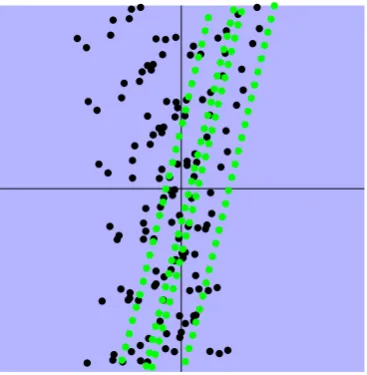
The figure is color coded; dark green boxes indicate SERAC external data sources, light green boxes contain SERAC gener-ated data and the red boxes symbolize major SERAC processes. The chain of processes begins with obtaining laser altimetry data, such as ICESat data from NASA’s satellite altimetry mission or ATM and LVIS data collected using NASA’s airborne systems, from NSIDC (National Snow and Ice Data Center). After con-verting the NSIDC data format to the SERAC format, the first processing step determines the location of surface patches, in-volving as many repeat missions from ICESat, ATM and LVIS. A surface patch constitutes the areal unit used in change detec-tion, size is about 1 km×1 km. Fig. 2 shows a typical surface patch.
laser altimetry data from NSIDC
surface patches find surface patches with repeat altimetry data
compute time series of surface elevations
FDM time series surface elevation
time series GIA rate
compute ice thickness changes related to ice dynamics
SMB time series time series of total, FDM, dynamic thickness changes
compute annual rates of thickness and mass changes at time series locations
total, dynamic, FDM, SMB annual change rates
interpolate from time series locations to grid
grids
compute spatial integrals to get ice sheet volume and mass balance rates
volume and mass balance change rates at individual glaciers, drainage basins,
or entire GrIS
Figure 1. Overview of SERAC with major computing modules (red boxes) and data sources (green boxes). Light green boxes are indicating SERAC internal data structure while dark green boxes are external data.
Figure 2. Example of a surface patch, approximate size 1 km ×1 km. The black dots are laser altimetry points of an ascend-ing ICESat track while green dots are from the descendascend-ing repeat track. The surface patch is located at the crossover of ascend-ing/descending tracks.
ful for estimating ice sheet mass balance or related sea-level rise. The conversion from elevation to mass starts with removing the vertical crustal motion due to Glacial Isostatic Adjustment (GIA) and the elastic crustal response to recent ice loading changes. The vertical crustal motion estimates for GIA are from (A et al., 2013) provided in a1◦
×1◦. The estimates range from 2.7 to 4.6 mm per year with errors negligible compared to the elevation change errors. The conversion from ice thickness to mass requires a firn densification model (FDM) to determine ice thickness changes related to ice dynamics, which can be converted to mass using the density of ice, typically 917 kg m−3
. The dynamic mass change is then combined with the surface mass balance (SMB) anomalies to obtain the total mass change. We refer to (Csatho et al., 2014) for details on the elevation change to mass change conversion. For the results shown in this paper we used the firn densifica-tion model from (Kuipers Munneke et al., 2015) and RACMO2.3 SMB estimates (No¨el et al., 2015).
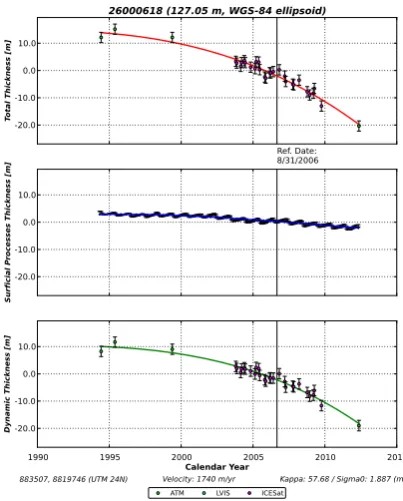
The surface elevation time series and the external data of FDM and GIA enter the modulecompute ice thickness changes related to ice dynamics. It produces time series of the total ice thickness, changes related to FDM, and determines changes related to ice dynamics (total change minus FDM change). Fig. 3 illustrates the results at a location near the grounding line of Zachariæ Is-strøm. The upper panel shows a time series of total ice thickness; thickness change related to surficial processes (FDM) are plotted in the middle panel and those caused by ice dynamics are shown in the lower panel. These results, together with the external SMB time series enters the next stage, calledcompute annual rates of thickness and mass changes at time series locations, that is iden-tical to the location of the original surface patches. We took the monthly SMB estimates from the climate model RACMO2/GR (No¨el et al., 2015) that is given on 11 km×11 km grid. This grid differs from the time series locations and the corresponding values have been found by nearest neighbor interpolation.
For convenience of computing, the final stage of SERAC takes place on regular grids. We first interpolate the annual rates com-puted at irregularly distributed time series locations to grids and then compute spatial integrals to get ice sheet volume and mass balance rates. The results are for the entire GrIS but they can also be analyzed on smaller regions, such as drainage basins or even individual outlet glaciers (Csatho et al., 2014).
3. METHOD FOR CORRECTING ASTER DEMS
This section presents a short synopsis of the method on how we correct ASTER DEMs that are introduced together with the more precise laser altimetry observations. For a more detailed descrip-tion the reader is referred to (Schenk et al., 2014).
We use AST 14 because GDEM is the average of all useful ASTER DEMS at a specific location and therefore not useful for detect-ing surface elevation changes over time. The reported vertical accuracy of AST 14 DEMs ranges from 15 m to 60 m. It is well-known that for surfaces covered by ice or snow, these values may become even larger, because gray level correlation is unreli-able if the image patches used for matching are nearly homoge-nous. Moreover, images with partial, undetected cloud coverage or ground fog may produce wrong elevations. In general, to ren-der stereoscopic DEMs useful for the computation of time-series of elevation changes it is important to correct them by aligning them to the more accurate laser altimetry points.
-20.0 26000618 (127.05 m, WGS-84 ellipsoid)
ATM LVIS ICESat
1990 1995 2000 2005 2010 2015
Calendar Year
883507, 8819746 (UTM 24N) Velocity: 1740 m/yr Kappa: 57.68 / Sigma0: 1.887 (m)
Figure 3. Time series of total ice thickness (upper panel), ice thickness changes due to surficial processes (middle panel) and caused by ice dynamics (lower panel) near the grounding line of Zachariæ Isstrøm.
parameters include a scale factor, 3 rotation angles, and 3 trans-lations. Since the rotation angles and the scale factor are rather small quantities, we can simplify the 3D similarity transforma-tion, using the differential rotation matrix, to obtain
2 expressed as a function of the transformation parameters;∆s, the scale;∆ω,∆ϕ,∆κ, the small rotation angles about thex−,y− andz−axes of the coordinated system; andxT, yT, zT, the co-ordinates of the translation vector. Thex, y, zare the original coordinates, that is,x and yare the grid post locations of the DEM, andz is its elevation. A traditional way to establish the seven unknown transformation parameters is using a set of known pointsx′, y′, z′(Ground Control Points, GCPs). Such GCPs have known coordinates in both coordinate systems. However, there are no identical points between laser altimetry and stereoscopic DEMs and all time epochs involved are different, that is, the re-lated observations are on different surfaces. The traditional way to use GCPs to calculate the transformation parameters does not work—a new approach is needed.
We begin by dividing the 3D transformation of Equation 1 into a horizontal and vertical transformation, assuming that the trans-formation parameters are small quantities and their products can be neglected. This assumption is certainly valid in our case where the transformation parameters are small corrections of DEMs.
The horizontal transformation is given as
x′=x∆s+y∆κ
−xT+x (2)
y′=
−x∆κ+y∆s−yT+y (3)
and contains the four parameters∆s(scale),∆κ(small rotation angle about thez−axis), andxT, yT(two horizontal shift
param-eters). For the vertical transformation we have
z′=x∆ϕ
−y∆ω−zT+z (4)
where ∆ω,∆ϕare the two rotation angles about the x−and
y−axes andzTis the vertical translation.
We apply first a 2D similarity transformation to align the ASTER DEMs horizontally, using control points and control features (dis-tinct lines identified and measured). Using control features is very advantageous as it is much easier to identify them unambigu-ously compared to points (Schenk et al., 2005). Control features include ridge crests and sudden changes in slope.
After the initial horizontal alignment we now turn to the cru-cial question on how to introduce vertical control information to transform the stereoscopic DEMs to the laser altimetry points, bearing in mind that there are no identical points between the two sets. Moreover, the time epochs and their related surface eleva-tions are different, too.
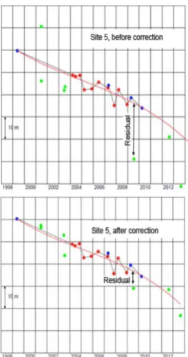
Fig. 4 shows the truncated time-series of elevation changes at site 5 (see Fig. 5 for site locations), for the time period 1997– 2013. including laser altimetry measurements (ATM = blue dots, ICESat = red dots) and stereoscopic DEMs (ASTER = green dots).
Looking closely at the laser altimetry points we notice increasing thinning from 2001 to 2006, followed by more stable elevations until 2011. Surface elevation changes are more deterministic than random, suggesting to fit an analytical curve to the points.
Our detailed study of 130 Greenland outlet glaciers revealed that dynamic thinning events of outlet glaciers occur normally over a short time period (exceptions exist) and they can be well de-scribed by a sigmoid curve. Therefore we fit the following alge-braic form of a sigmoid curve
h=p−d(t−a)
1 +b(t−a)2 +c (5)
to the ATM and ICESat points. In this equation,trefers to time,
his the elevation relative to August 31, 2006 anda, b, c, dare the four parameters that have to be determined during the curve fitting process.
Figure 4. Elevation time series for site 5 near the grounding line of Zachariæ Isstrøm (circled in red in Fig. 5) before the DEM correction is applied (upper panel) and after the DEM correction (lower panel). Altimetry observations are from ICESat (red) and ATM (blue). Green dots mark elevations derived from ASTER DEMs.
the three unknown correction parameters of every DEM we need to repeat the process at least at two more time-series locations, preferably many more to formulate an adjustment problem.
Suppose we haventime-series,n > 3. In this case, the three correction parameters per DEM can be found by a least-squares adjustment. Equation 4 is slightly rearranged to become a linear observation equation
ei=xi∆ϕ−yi∆ω−zT+zi−z′i (6)
witheithe residual at locationi,∆ϕ,∆ωthe rotation angles,zT
the vertical shift parameter,xi, yi the coordinates at locationi
andzi−zi′the observed error.
Figure 5 illustrates the procedure. The original DEM (black) is transformed to the corrected position (red) by two small rotational angles, ∆ω,∆ϕ, about the x and y—coordinate axes and the vertical shift,zT. The linear error model is a first approximation and future research has to address more complex, non-linear error models.
We summarize the procedure to correct stereoscopic DEMs for elevation errors, assuming that a horizontal registration has been accomplished first, for example by using Equations 2 and 3 on stationary points and lineal features. Lineal features offer the ad-vantage of improved identification and localization but require a more sophisticated transformation algorithm than presented in Equations 2 and 3. Since we focus in this paper on correcting el-evations, we do not elaborate further on the horizontal alignment.
erence frame, here WGS-84.
2. Select locations with repeat ICESat, ATM and LVIS laser altimetry data and stereoscopic DEMs to be corrected.
3. Compute time-series with SERAC at the selected locations and fit a sigmoid curve through the laser altimetry points.
4. Calculate the differences of DEM points to the fitted curve and enter them as observations into Equation 6 to compute the three DEM correction values (2 small angles∆ω,∆ϕ) and absolute elevation correction (zT).
5. Repeat the time-series calculation with the corrected DEMs as a final check.
Finally, the lower panel of Fig. 4 presents the time-series of eleva-tion changes after correcting the stereoscopic DEMs. The red line is the same polynomial curve as in the upper panel fitted through the laser altimetry points. We observe that the DEM points are now randomly distributed about the curve. However, their spread is noticeably larger than the red and pink laser altimetry points, reflecting their lower precision.
4. RESULTS
We present detailed examples of the Zachariæ Isstrøm (ZI) in northeast Greenland, involving ICESat and ATM laser altime-try data, together with DEMs obtained the Advanced Spaceborne Thermal Emission and Reflection Radiometer (ASTER) and stereo aerial photogrammetry. Zachariæ Isstrøm is one of the main out-lets of the Northeast Greenland Ice Stream (NEGIS, Fig. 5). NEGIS is the only large ice stream of the GrIS, a linear body of fast-moving ice that penetrates 700 km into the interior of Greenland. Its drainage basin represents 12 % of the GrIS and contains a sea-level rise equivalent of 1.1 m (Mouginot et al., 2015). Zachariæ Isstrøm is currently undergoing rapid changes in surface eleva-tion and ice velocity, manifesting as ice front retreat, accelerating speed-up and thinning (Khan et al., 2014, Mouginot et al., 2015).
We fused the altimetry and stereo DEM record (Fig. 5) to examine the elevation changes of Zachariæ Isstrøm between 1978-2013.
The fused elevation change data set allow the characterization of glacier elevation changes at different spatial and temporal scales. The SERAC times series provided the first accurate measure-ments of the accelerating thinning (Csatho et al., 2014). The thin-ning is mostly due to ice dynamic processes, i.e., the acceleration of ice flow with a minimum contribution from increasing surface melt (Fig. 3).
Figure 5. Location map of data combined for elevation change reconstruction. Elevation data set includes ICESat (purple lines) and ATM (green lines) altimetry and ASTER DEMs (a total of 10; June 21, 2001 (red box); July 19, 2009 (orange box) and August 23, 2013 (blue box) are shown). Small yellow circles mark surface patches used for DEM correction. Elevation change time series for site 5 (large red circle) are presented in Fig. 4. Central flow line profile, shown Fig. 9, is marked by red line. Thick black line is 2013 calving front. Small map shows location of Zachariæ Isstrøm (ZI) on ice velocity map from Rignot and Mouginot (2012).
Figure 6. Statistics and errors of DEMs used in this study.
5. CONCLUDING REMARKS
Zachariæ Isstrøm, one of the three outlet glaciers draining ice from the North East Greenland Ice Stream (NEGIS), has expe-rienced accelerating thinning and speed-up leading to increasing mass loss during the last decades (Khan et al., 2014, Mouginot et al., 2015). To investigate the mechanisms controlling ice dy-namical changes, we reconstructed its elevation change history between 1978 and 2014. Our analysis shows accelerating thin-ning between 1974-2014 within 25 km distance from the 1996 grounding line, in a region where that glacier’s bed is the deep-est at 600 meter below sea level. This finding is consistent with acceleration and thinning initiated by ice loss near the grounding line, most probably caused by ocean warming (Mouginot et al.,
Figure 7. Statistics and errors for the 18 SERAC times series used as control information for the fusion and the correction process. Locations are shown by small yellow circles in Fig. 5.
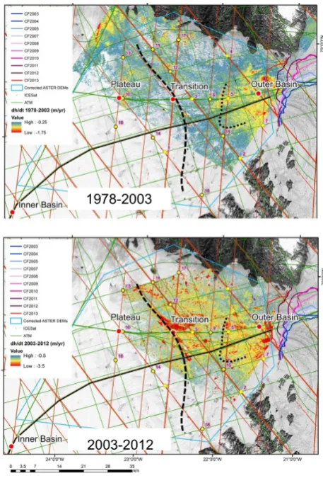
Figure 8. Upper panel: elevation change between 1978 (aerial photogrammetry DEM) and 2003 (corrected ASTER DEM). Lower panel: elevation change between 2003 and 2012 (both corrected ASTER DEMs). Warm, red colors indicate largest thin-ning. Colored lines mark calving front positions and dashed black lines indicate large changes in bedrock elevation.
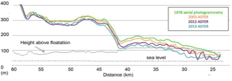
Figure 9. Elevation change along the central flow line from 1978 to 2013 from aerial photogrammetry DEM (1978) and corrected ASTER DEMs (2003, 2012, 2013.
.
in discrete steps from the calving front toward inland. Therefore, we suggest that bedrock topography or processes acting along the entire glacier, such as changes in lateral drag or ice viscosity, also influence Zachariæ Isstrøm’s response to changing environmental conditions.
Our analysis of ICESat time series shown that dynamic thinning extended as far as 100 km inland by 2007 (Csatho et al., 2015), indicating that an increasingly large region of the glacier is be-coming vulnerable to further ocean warming and air tempera-ture increase. We detected a pattern of ”blockwise” thinning, i.e., separate large regions thinning with uniform rates (Fig. 9). This is markedly different from a simple inland propagating dif-fusion signal, possibly caused by rapid ice loss at the ground-ing line and observed for example on Kangerlussuaq Glacier in east Greenland (Schenk et al., 2014). We speculate that major bedrock topographic features act as barriers for inland propaga-tion of thinning on Zachariæ Isstrøm. A comparison of our de-tailed thickness changes history with numerical modeling results from the Ice Sheet System Model (Larour et al., 2012, Schlegel et al., 2014) suggests that while most of the observed rapid thinning is likely caused by grounding line retreat, a dynamic response of ice flow to surface mass balance variations might also play an important role (Csatho et al., 2015).
6. ACKNOWLEDGEMENT
We thanks Michiel van den Broeke and Peter Kuipers Munneke (Institute of Marine and Atmospheric Research, Utrecht Univer-sity, Utrecht, The Netherland) for FDM and SMB data sets, Kurt Kjær (Centre for GeoGenetics, Natural History Museum, Univer-sity of Copenhagen, Copenhagen, Denmark) for the DEM gener-ated from 1978 aerial photographs and Greg Babonis (Depart-ment of Geology, University at Buffalo, Buffalo, NY) for post processing SMB and FDM data.
REFERENCES
A, G., Wahr, J. and Zhong, S., 2013. Computations of the vis-coelastic response of a 3-D compressible Earth to surface load-ing: an application to Glacial Isostatic Adjustment in Antarctica and Canada.Geophysical Journal International192(2), pp. 557– 572.
Csatho, B., Larour, E., Schenk, A., Schlegel, N. and Duncan, K., 2015. Investigation of controls on ice dynamics in Northeast Greenland from ice-thickness change record using Ice Sheet Sys-tem Model (ISSM). Abstract C51E-07 presented at 2015 AGU Fall Meeting, AGU, San Francisco, CA.
Duncan, K., Rezvanbehbahani, S., Van Den Broeke, M. R., Si-monsen, S. B., Nagarajan, S. and Van Angelen, J. H., 2014. Laser altimetry reveals complex pattern of Greenland Ice Sheet dynam-ics. Proceedings of the National Academy of Sciences111(52), pp. 18478–18483.
Khan, S. A., Kjær, K. H., Bevis, M., Bamber, J. L., Wahr, J., Kjeldsen, K. K., Bjørk, A. A., Korsgaard, N. J., Stearns, L. A., Van Den Broeke, M. R., Liu, L., Larsen, N. K. and Muresan, I. S., 2014. Sustained mass loss of the northeast Greenland ice sheet triggered by regional warming. Nature Climate Change 4(4), pp. 292–299.
Kuipers Munneke, P., Ligtenberg, S. R. M., No¨el, B. P. Y., Howat, I. M., Box, J. E., Mosley-Thompson, E., McConnell, J. R., Stef-fen, K., Harper, J. T., Das, S. B. and Van Den Broeke, M. R., 2015. Elevation change of the Greenland Ice Sheet due to surface mass balance and firn processes, 1960–2014. The Cryosphere 9(6), pp. 2009–2025.
Larour, E., Seroussi, H., Morlighem, M. and Rignot, E., 2012. Continental scale, high order, high spatial resolution, ice sheet modeling using the Ice Sheet System Model (ISSM). Journal of Geophysical Research: Atmospheres (1984–2012).
Mouginot, J., Rignot, E., Scheuchl, B., Fenty, I., Khazendar, A., Morlighem, M., Buzzi, A. and Paden, J., 2015. Fast retreat of Zachariæ Isstrøm, northeast Greenland. Science350(6266), pp. 1357–1361.
No¨el, B., van de Berg, W. J., van Meijgaard, E., Kuipers Munneke, P., van de Wal, R. S. W. and Van Den Broeke, M. R., 2015. Summer snowfall on the Greenland Ice Sheet: a study with the updated regional climate model RACMO2.3. The Cryosphere Discussions9(1), pp. 1177–1208.
Schenk, T. and Csatho, B., 2012. A new methodology for detect-ing ice sheet surface elevation changes from laser altimetry data. Geoscience and Remote Sensing, IEEE Transactions on50(9), pp. 3302–3316.
Schenk, T., Csatho, B., Van Der Veen, C. and McCormick, D., 2014. Fusion of multi-sensor surface elevation data for improved characterization of rapidly changing outlet glaciers in Greenland. Remote Sensing of Environment149, pp. 239–251.
Schenk, T., Csatho, B., Van Der Veen, C. J., Brecher, H., Ahn, Y. and Yoon, T., 2005. Registering imagery to ICESat data for measuring elevation changes on Byrd Glacier, Antarctica. Geo-physical Research Letters32(23), pp. L23S05.