COMPARISON OF HIGH AND LOW DENSITY AIRBORNE LIDAR DATA FOR
FOREST ROAD QUALITY ASSESSMENT
K. Kiss a*, J. Malinen b, T. Tokola c
University of Eastern Finland, Faculty of Science and Forestry, School of Forest Sciences, P.O. Box 111 (Yliopistokatu 7), FI-80101 Joensuu, Finland.
a [email protected] b [email protected]
Comission ThS 2
KEY WORDS: forest road, road quality, forestry, LiDAR, ALS
ABSTRACT:
Good quality forest roads are important for forest management. Airborne laser scanning data can help create automatized road quality detection, thus avoiding field visits. Two different pulse density datasets have been used to assess road quality: high-density airborne laser scanning data from Kiihtelysvaara and low-density data from Tuusniemi, Finland. The field inventory mainly focused on the surface wear condition, structural condition, flatness, road side vegetation and drying of the road. Observations were divided into poor, satisfactory and good categories based on the current Finnish quality standards used for forest roads. Digital Elevation Models were derived from the laser point cloud, and indices were calculated to determine road quality. The calculated indices assessed the topographic differences on the road surface and road sides. The topographic position index works well in flat terrain only, while the standardized elevation index described the road surface better if the differences are bigger. Both indices require at least a 1 metre resolution. High-density data is necessary for analysis of the road surface, and the indices relate mostly to the surface wear and flatness. The classification was more precise (31–92%) than on low-density data (25–40%). However, ditch detection and classification can be carried out using the sparse dataset as well (with a success rate of 69%). The use of airborne laser scanning data can provide quality information on forest roads.
1. INTRODUCTION
Forest roads enable easy access to harvesting sites, allowing the use of efficient harvesting machinery and shorter forest transportations. Forest roads offers also possibilities to mechanized silvicultural operations, recreation, the collection of non-wood products and access for protective services, such as firefighting and rescue operations. The road condition is essential; roads with higher bearing capacity can be used by heavier vehicles without causing further damage. Uneven road surfaces, ruts and holes require a slower driving speed, may damage the vehicles or accumulate water in them (Haavisto et al. 2011).
In Finland, the forest road network has been built to a great extent from the 1970s to the 1990s, and the level of new road construction has since diminished to under 20 per cent of the top years. At the same time, the forest road network is ageing, leading to increased maintenance and renovation needs. The currently used inventory methods for forest road quality demand visits to the site, and most often the inventory is based on subjective classification of visible road condition. The forestry applications of Airborne Laser Scanning (ALS) are mainly focused on forest inventories. Low resolution ALS data (less than 1 pulse per m2) is used in the Area-Based Approach to estimate forest variables
*Corresponding author
using ALS-based predictors (Næsset 2002; Maltamo et al. 2014; Peuhkurinen et al. 2011). The method is widely used in practice, although tree species recognition is not totally solved.
The Individual Tree Delineation (ITD) uses dense laser scanning data. Dense data is at least 5 pulses per m2, but often 10 pulses per m2 data are used. The dimensions of trees can be measured from the ALS data and aggregated to the desired level (Vauhkonen at al. 2011). It allows individual trees and tree species to be identified, and its accuracy is similar to the previous method (Maltamo et al. 2014).
Studies concerning road construction (Ghajar et al. 2013), maintenance (Coulter et al. 2006) and environmental concerns affecting the placement of roads in forests (Grayson et al. 1993; Rummer et al. 1997; Forsyth et al. 2006; Jordán and Martínez-Zavala 2008.) show big variety. Forest road condition can be evaluated using remote sensing technology. Zhang (2008) was working on a system in the United States that can evaluate unpaved roads without field surveys.
Recent studies focus on road extraction from LiDAR data. White et al. (2012) extracted roads in forested areas which were partially covered with different dense canopies. Azizi et al. (2014) worked on automatized road extraction, and could locate roads with 63% accuracy. Road quality (Kiss et al. (2015), geomatics and grade of forest roads have been studied as well (Craven and Wing 2014). Haavisto et al. (2011) and Uusitalo et al. (2012) were testing how to calculate the bearing capacity of peatlands from ALS data. Bearing capacity was calculated for quite large pixel sizes based on the volumes of the trees and their relative elevations. The method requires further development, but it could be useful in future for gathering information relevant to wood harvesting and transportation.
High-density ALS data is still expensive, but multiple-use of the data can reduce its cost. In forest inventory for individual tree delineation and species recognition (Vauhkonen et al. 2012) or in geomorphological modelling (Höfle and Rutzinger 2011) the required datasets have a similar density to the ones for road assessment. Another possibility for cost-reduction is the use of unmanned aerial vehicles (UAVs) (Wallace et al. 2012). UAVs can fly above roads and map them more efficiently than laser scanning inventories which cover the whole forest area. These provide the opportunity for future economic use.
The current work was testing the applicability of different pulse density ALS data so as to assess forest road conditions, focusing on the structural condition, surface wear, flatness and drying of the roads. Both ALS data have been recorded for forest inventory purposes. Laser scanning can lead to cost reduction in the road inventory by locating problematic sections on the roads without spending time and money on field inspection of the roads.
2. MATERIALS 2.1 Field data
The field data was collected based on the accepted Finnish road quality standards. Two study areas have been inventories. The first data was collected in August 2013 at Kiihtelysvaara, the second dataset in July 2014 at Tuusniemi, Finland.
The first study area has slight topographic differences, the roads steepness does not exceed 1.7° per 10 m, and the total length of forest roads in the area is 9.7 km. No recent road maintenance has been observed. The second study area has greater elevation differences (up to 20% of road steepness) and recent road maintenance has been carried out in certain locations. Respectively thirteen and fifty field plots sampled the roads (2–3 plots per road sections) and 10 m on either side of them.
Based on the Finnish national road quality standards (Metsätehon raportti 2008), the following categories were included in the inventory: structural condition, seasonal damage, drying (including surface wear, ditches and side bumps), geometry, design and visibility, coppicing, bridges, and flatness. For each of these categories, each observation was placed in one of three quality classes: good (3), satisfactory (2), or poor (1). Note that poor category roads have been inventoried only in the second study area.
Road surface quality and the ditching system were at the focus of the research; therefore, the structural condition, drying, surface wear and flatness categories were taken for further analysis.
2.2 Airborne laser scanning data
The high-density ALS data for the first study were collected on 26 June 2009 using an Optech ALTM Gemini laser scanning
system, and the scanning took place from 600 m above ground level. The scanner had a field of view of 26°, a pulse repetition frequency of 100 kHz, which resulted in a sampling density of about 12 measurements·m2. The scanning strip had a width of approximately 320 m and 55% of side overlap. The time gap between the field data and LiDAR data has been acknowledged, as it can affect the road condition, and this will be discussed later.
The low-density ALS data for the second study area was collected on 23 July 2014 by Leica ALS50-II laser scanning system from about 2000 m above ground level. It had a 20° to the field view,114 kHz pulse repetition frequency, the average sampling density was 1.1 pulses per m2 with a 20% or side overlap. There is no significant time gap between the ALS and field data.
Digital elevation models (DEMs) were created for further analysis. DEMs have been interpolated in resolutions 2 m, 1 m, 0.5 m, 0.25 m and 0.10 m. The last of many echoes and only echoes were used during the interpolations of surface, while the first of many echoes and only echoes were used in vegetation modelling, which was useful mostly to map ditches.
3. METHODS
The research focused on road surface and ditch system conditions. The road surface condition is determined by different factors: surface wear, structural condition, seasonal damage and flatness. Tyre tracks, holes or improper drying can be observed if any or all of these are in poor condition. Secondly, the ditch systems were identified and assessed. Road-side vegetation can obstruct proper drainage if it grows in the ditches.
Currently, there are no existing accepted methods for road quality assessment using ALS data. This paper discusses how to use various existing tools in order to assess road quality. Several different indices have been calculated and compared using the ALS point cloud and the different resolution DEMs. The road centrelines data was available from the Finnish Transport Agency (2013). The widths of the roads were obtained from field measurements.
The elevation values were assessed to determine topographic variations in the roads. To assess the road surface, 3m by 3 m squares were defined around the field data point to cover the road surface. The indices were calculated to these squares, compared and validated by using the field data about structural condition, seasonal damage, surface wear and flatness.
An ArcGIS extension, Land facet corridor analysis (Jenness Enterprises 2013) was used for the surface analysis. The following indices can analyse landscape conditions. The topographic position index (TPI) and standardized elevation index (SE) can be calculated from the DEMs. It provides a simple and repeatable method for classifying the landscape into slope position and/or landform categories. The original application of the index was to determine positive landforms like peaks, mountains, neutral landforms such as plains or plateaus, and negative landforms such as valleys or canyon. In this research, we applied the index on a smaller scale due to the available ALS data.
the neighbourhoods (Equation 1). The SE index is very similar to the TPI index; it divides the TPI by the standard deviation of the neighbourhoods (Equation 2). The SE index is expressed in standard deviations, which means that an SE index of 1 of a cell would mean that this particular cell is 1 standard deviation higher than the mean elevation in the neighbourhoods. While positive values mean higher locations, negative values mean the cells are lower than their neighbourhoods.
��
�= �
�−
∑ �� � �=1� (1)
�
�=
��−∑��=1�� �
� (2)
where ��= height
� = cells in the neighbourhood
� = standard deviation of the selected neighbourhood
When the TPI and SE index were used for road quality assessment, they were applied on a small scale, making it possible to locate small unevennesses in the road as being lower (e.g., holes) or higher (e.g., stones, vegetation) than their environment.
The most important property of the indices is their neighbourhood. The calculated indices depend on the size and shape of the neighbourhoods taken into consideration. Setting the proper scale is essential. Smaller neighbourhoods can show smaller differences, whereas broader neighbourhoods will map large landform efficiently, but do not show the smaller depressions or peaks. The neighbourhoods can be in several different shapes, for example circle, square, ring, etc. A three-metre square shape has been chosen for the analysis of the road quality.
The surface can be assigned to various categories based on its degree of slope and index values. It has been used for ditch detection. Ditches and non-ditches were classified in 3 m wide and 20 m long corridors parallel with the central line of the road on both sides. This categorization has been used for ditch detection.
4. RESULTS
The spatial resolution of DEMs highly depends on the density of the available ALS point cloud. In the second study area, the interpolated DEMs were in poorer resolution due to the sparse dataset.
The neighbourhood size for the indices had been tested between up to 20 cells. Bigger neighbourhoods mean longer calculation times and their usability for road quality was reduced as well, because the bigger neighbourhoods averages the smaller differences on the surface. It is possible to use bigger neighbourhood sizes only for ditch detection purposes; there is no need to increase calculation times if the detection can be done on a smaller neighbourhood as well. Considering these, a two metre radius neighbourhood have been used, which meant more cells at better resolution, and fewer cells at lower resolution.
The TPI index reflects more the original differences (for example slope) of the road than does the SE index. The latter index is less dependent, and therefore showed better results in road surface condition and ditch detection as well.
4.1 Locating ditches
Ditches and the surrounding vegetation can be clearly detected visually from the high resolution ALS data. The classification of ditches in the low pulse density dataset was least successful. Figure 1 and Figure 2 show the difference between the DEMs generated from the two datasets in different resolutions. Figure 2 shows that a ditch was identified only on one side of the road. If the laser pulse did not hit the bottom of the ditch, the ditches cannot be identified or they are classified as poor quality ditches, which hinders the classification results.
TPI index was calculated to detect the ditch systems. Negative TPI values define negative landforms compared to their neighbourhood; therefore, by setting a threshold value it was possible to classify the landscape into ditches and non-ditches using the index.
Figure 1. Road cross-section of DEMs interpolated from high-pulse density ALS dataset. All resolutions represent the same
cross section.
Figure 2. Cross-section of DEMs interpolated from low-pulse density ALS dataset on resolutions 1 m
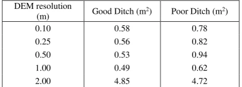
DEM resolution
(m) Good Ditch (m2) Poor Ditch (m2)
0.10 0.58 0.78
0.25 0.56 0.82
0.50 0.53 0.94
1.00 0.49 0.62
2.00 4.85 4.72
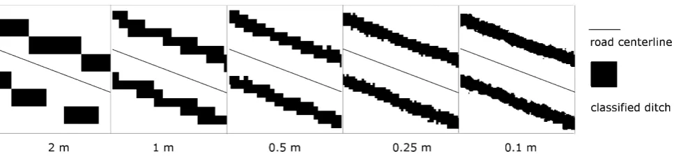
Figure 3 Ditch and non-Ditch classification at several resolutions
Ditch systems were successfully detected in all resolutions up to 1 metre. 2-merer resolution did not result in continuous ditches even if the ditch quality was good (Figure 3). Ditches were classified into two categories: good and poor ditches. The latter included both satisfactory and poor quality ditches. The percentage of the ditch area has been evaluated based on the different resolutions to determine whether the section has a good ratio of ditches or not. The standard error of mean was low in all cases except in the 2 m resolution. (Table1) The 0.25 m cells provided the best detection results. Leave-out-out cross-validation confirmed that 69% of the ditches were classified correctly, and the difference between the ditch sizes was statistically significant on the assumption of equal variance.
4.2 Road surface analysis
TPI and SE indices were calculated and verified against the field data of structural condition, surface wear quality and flatness. The assessment of road surface quality gave essentially different results for the two datasets.
Figure 1 shows that at the resolution of 2m and 1m the inequalities of the road surface are not easily detectable, only the general profile of the road. Table 2 shows the mean values for good and satisfactory surface wear at each resolution. The standard error of mean (SEM) was high for 1 m and 2 m resolutions. In the case of higher resolutions, SEM was low and also the difference between the quality classes were statistically significant based on T-test. The difference between the quality classes at 0.1 m and 2m resolution did not show statistical
0.25 Satisfactory -0.0064 0.0061
0.50 Good -0.0399 0.0222
0.50 Satisfactory -0.0541 0.0244
1.00 Good 0.1241 0.1204
1.00 Satisfactory -0.0516 0.1145
2.00 Good -0.1440 0.2322
2.00 Satisfactory -0.0423 0.2266 Table 2. Evaluation of SE index to determine the surface wear
condition.
The cross-validation (Table 3) confirms that the classification was more successful at bigger resolutions and on the high pulse density dataset. The low point density dataset has lower success in classification as the dataset contained three quality classes
inventoried during the field work, while the other data contained only two classes. At higher resolutions, the SE index showed better classification than the TPI; however, it was the opposite in case of low resolution data.
The index values have greater variance when the road quality is poorer. The standard deviation of the index values gave better results than their mean value at most moving window sizes. This means that the good quality roads have fewer or smaller elevation differences than the satisfactory quality roads, and the poor quality roads have the biggest or most elevation differences. The surface wear was classified with the best results by using the dense dataset. The quality classes were determined correctly up to 92% at a resolution of 0.25 m. The structural condition was the best mapped at resolutions of 0.5 m and 1 m, and the flatness at 0.5 m. The 0.1 m resolution did not lead to better classification than the lower resolutions.
Table 3. Cross-validation of the classification of road surface quality shows the percentage of sections has been correctly classified. The classification was based on TPI and SE indices
in resolutions from 0.1 m to 1 m. The high pulse-density and low pulse density ALS data were both tested.
5. DISCUSSION
The research assessed two airborne laser scanning datasets, each with a different point density, in order to determine which can be used for road quality evaluation. The three-year gap between the data collection and the field inventory is a weakness of the high density ALS data. The road conditions could have changed during that time period. At the current location, the change only means that the road condition could have deteriorated, because there was no road maintenance carried out.
resolution; however, they provided information about the structural condition as well at smaller resolutions.
The sparse dataset had limited resolution possibilities, and it had lower precision in classifying the road surface parameters compared to the dense dataset. On the other hand, the sparse dataset could provide information about the ditch systems by detecting its presence. The detection of ditches worked well in both datasets up to 1 m resolution.
It is important to note that bigger size ditches are not always better than the smaller sized ones. Different soil types or geomorphological condition may require ditches of different size and depth to obtain good dryings of the roads. The size and depth of the ditches are determined by the slope of the ditch, the area to be drained, the estimated intensity, the volume of run-off and the amount of sediment that can be expected to be deposited in the ditch during periods of flow (FAO, 1989).
Choosing the proper resolution for the road quality assessment is challenging. According to James et al. (2007), 12 pulse per m2 dense data was required to determine the depth of gullies, but sparser data can be used in locating them. This research shows similar results: the ditches were mapped more precisely at higher resolutions. The resolution of DEMs is also critical in case of road extraction from LiDAR data (White et al. 2010 and Azizi et al. 2014). Road curves and grades can be assessed even from sparse (1.12 pulse per m2) airborne scanning dataset (Craven and Wing, 2014).
Dense canopy cover would limit the proposed method. The laser pulses cannot penetrate through dense vegetation or canopy cover which would limit the usage of the application especially in the tropics. Furthermore, the performance of the application need to be tested on mountain areas where the elevation differences are significant.
The continuation of the research can introduce a reference surface. It would reduce the topographical effect influenced by the indices (mostly in the case of TPI). It would be especially beneficial for the TPI index. It can increase the usability of low resolution laser scanning data as well, which could make the method cheaper in practical use. Furthermore, it would contribute to its use on mountainous terrains.
In conclusion, the methods were successfully tested on both datasets. Road surface quality can be detected on high density ALS data while the ditch system can be detected on the sparse dataset as well. The results provide the opportunity that, after further development, airborne laser scanning data can be used for road quality assessment in forest road management.
REFERENCES
Azizi, Z., Najafi, A., Sadeghian, S. 2014. Forest road detection using LiDAR data. J. For. Res. 25(4), pp. 975-980.
Coulter, ED., Sessions, J., Wing, MG. 2006. Scheduling forest road maintenance using the analytic hierarchy process and heuristics. Silva Fenn. 40(1), pp. 143-160.
Craven, M., Wing, M. 2014. Applying airborne LiDAR for forested road geomatics. Scand. J. For. Res. 29(2), pp. 174-182.
FAO. 1989. Watershed management field manual. Road design and construction in sensitive watersheds. FAO Conservation Guide 13/5, Food and Agriculture Organization of the United
Forsyth, AR., Bubb, KA., Cox, ME. 2006. Runoff, sediment loss and water quality from forest roads in a southeast Queensland coastal plain Pinus plantation. For. Ecol. Manage. 221(1–3), pp. 194-206.
Ghajar, I., Najafi, A., Karimimajd, AM., Boston, K., Torabi, S. 2013. A program for cost estimation of forest road construction using engineer’s method. For. Sci. Technol. 9(3), pp. 111-117.
Grayson, RB., Haydonb, SR., Jayasuriyab, MDA., Finlayson, BL. 1993. Water quality in mountain ash forests — separating the impacts of roads from those of logging operations. J. Hydrol.
150(2–4), pp. 459-480.
Haavisto, M., Kaakkurivaara, T., Uusitalo, J. 2011. Älykkyyttä puunkorjuun suunnitteluun — Laserkeilaus- ja paikkatietoaineistojen hyödyntämismahdollisuudet turvemaaleimikon ennakkosuunnittelussa. Working papers of the Finnish Forest Research Institute 201. http://www.metla.fi/julkaisut/workingpapers/2011/mwp201.htm (5 May 2014). [In Finnish.]
Höfle, B., Rutzinger, M. 2011. Topographic airborne LiDAR in geomorphology: a technological perspective. Zeitschrift fur Geomorphologie 55(2 Supplementary Issue), pp. 1-29.
James, A., Watson, D., Hansen, W. 2007. Using LiDAR data to map gullies and headwater streams under forest canopy: South Carolina, USA. Catena 71(1), pp. 132-144.
Jenness Enterprises. 2013. Land Facet Corridor Analysis. http://www.jennessent.com/arcgis/land_facets.htm (2 Jan 2014).
Jordán, A., Martínez-Zavala, L. 2008. Soil loss and runoff rates on unpaved forest roads in southern Spain after simulated rainfall. For. Ecol. Manage. 255(3–4), pp. 913-919.
Kiss, K., Malinen, J., Tokola T. 2015. Forest road quality control using ALS data. Can. J. For. Res. 45(11): pp. 1636-1642.
Maltamo, M., Næsset, E., Vauhkonen, J. 2014. Forestry applications of airborne laser scanning — concepts and case studies. Managing Forest Ecosystems 27. pp. 464.
Metsätehon raportti. 2008. Metsäteiden kuntoinventoinnin ja kuntotiedon hyödyntämisen toimintamalli: 202: pp. 23–36. Liite II. [In Finnish.] www.metsateho.fi/wp-content/uploads/2015/02/Raportti_202_AK.pdf (2 Aug 2013).
Rummer, RB., Strokes, B., Lockaby, G. 1997. Sedimentation associated with forest road surfacing in a bottomland hardwood ecosystem. For. Ecol. Manage. 90(2), pp. 195-200.
Uusitalo, J., Kaakkurivaara, T., Haavisto, M. 2012. Utilizing airborne laser scanning technology in predicting bearing capacity of peatland forest. Croatian Journal of Forest Engineering 33(2), pp. 329-337.
Wallace, L., Lucieer, A., Watson, C., Turner, D. 2012. Development of a UAV-LiDAR system with application to forest inventory. Remote Sens. 4(6), pp. 1519-1543.
White, RA., Dietterick, BC., Mastin, T., Strohman, R. 2010. Forest roads mapped using LiDAR in steep forested terrain.
Remote Sens. 2(4), pp. 1120-1141.
Zhang, C. 2008. Monitoring the condition of unpaved roads with remote sensing and other technology. Final Report for US DOT DTPH56-06-BAA-0002, Geographic Information Science Center of Excellence, South Dakota State University, National
Transportation Library.
http://ntl.bts.gov/lib/42000/42300/42378/FinalReport.pdf (12 Sep 2013).