T H E J O U R N A L O F H U M A N R E S O U R C E S • 47 • 4
Income Taxes
Are the Wages of Dangerous Jobs More
Responsive to Tax Changes than the Wages
of Safe Jobs?
David Powell
A B S T R A C T
Income taxes distort the relationship between wages and nontaxable amen-ities. When the marginal tax rate increases, amenities become more valu-able as the compensating differential for low-amenity jobs is taxed away. While there is evidence that the provision of amenities responds to taxes, the literature has ignored the consequences for job characteristics which cannot fully adjust. This paper compares the wage response of dangerous jobs to the wage response of safe jobs. When tax rates increase, we should see the pretax compensating differential for on-the-job risk increase. Em-pirically, I find large differences in the wage response of jobs based on their riskiness.
I. Introduction
The theory of compensating differentials has been well-established since the writings of Adam Smith in 1776. Nonwage amenities should impact work-ers’ wages, and much empirical research has been dedicated to studying the rela-tionship between wages and amenities. There is little research studying how these compensating differentials interact with income and wage taxes. While nonwage
David Powell is an economist at RAND. He is grateful to David Autor, Arthur Campbell, Tom Chang, Jesse Edgerton, Michael Greenstone, Tal Gross, Jon Gruber, Jerry Hausman, Helen Hsi, Konrad Menzel, Whitney Newey, Amanda Pallais, Jim Poterba, Nirupama Rao, Hui Shan, and Carmen Taveras for their comments. He thanks Dan Feenberg and Inna Shapiro for their help with NBER’s Taxsim program. Katharine Earle of the U.S. Census Bureau provided invaluable industry crosswalks. Special thanks to Suzanne Marsh of the National Institute for Occupational Health and Safety for providing detailed occu-pational fatality data. With the exception of restricted fatality numbers, the data used in this article can be obtained beginning May 2013 through April 2016 from David Powell; 1776 Main St., Santa Monica, CA 90407, dpowell@rand.org. This research was supported by the National Institute on Aging, Grant Number P01-AG05842.
[Submitted June 2011; accepted January 2012]
amenities are untaxed, the compensating differential is subject to taxation. When tax rates change, the pretax wages of jobs with different nonwage amenities must shift differentially. Consequently, observed compensating differentials are a function of tax rates. We should observe heterogeneity in the incidence of income taxes based on the amenity level of the job. This paper provides theoretical and empirical evi-dence for the relationship between compensating differentials and marginal tax rates. This paper compares the wage response of jobs with different levels of amenities to legislative tax changes. I focus on industries with varying on-the-job hazard rates for three reasons. First, occupational safety is easy to measure. Second, a vast lit-erature has studied the existence and magnitude of compensating differentials with respect to occupational hazards. Individuals working in risky jobs should be com-pensated for the additional risk with higher wages. Third, while many amenities likely respond to tax changes, some amenities cannot fully adjust and are simply fixed characteristics of a job. Occupational safety is an example where the most dangerous jobs never become as safe as the safest jobs, regardless of the tax envi-ronment. Risk rates may adjust to some extent, but it is still possible to measure a compensating differential under different tax regimes.
This paper looks at how the pretax wages of dangerous jobs respond to tax changes relative to the pretax wages of safe jobs. When marginal tax rates (τ) increase, the compensating differential associated with dangerous jobs is taxed away. The key parameter is the marginal net-of-tax rate, the fraction of an additional dollar of earnings that a worker keeps. If a high risk job pays an extra $1 as a compensating differential, the worker keeps $(1−τ). Workers are paid in taxable earnings and nontaxable amenities, such as safety. When tax rates increase, all workers are im-pacted, but workers paid disproportionately in monetary wages are affected more. In response, the pretax compensating differential must increase, implying that the wages of the dangerous jobs must increase more than the wages of the safe jobs for a given difference in risk.
It is well-known that individuals and firms respond to tax changes. Taxes distort individual labor supply decisions and occupational choices. Similarly, firms may alter the generosity of their nontaxable amenities in response to taxes. Both of these phenomenon have been studied in the tax literature. However, these effects do not fully encapsulate the magnitude of the distortion resulting from taxes. Nontaxable amenities cannot completely adjust in response. Jobs have some fixed characteristics which are incapable of responding to tax changes. Instead, wages must adjust. Con-sequently, taxes may distort the cross-industry relationship between pretax wages.
source of distortion. To my knowledge, this is the first paper to estimate the differ-ential incidence of income tax rates based on variation in an amenity.
I use the 1983–2002 March Current Population Survey (CPS) with Bureau of Labor Statistics (BLS) injury data and National Institute for Occupational Safety and Health (NIOSH) fatality data to estimate the relationship between wages, injury and fatality rates, and marginal net-of-tax rates (1−τ). Because tax rates are a
func-tion of wages, I use an IV strategy similar in spirit to Currie and Gruber (1996a,b) where identification originates solely from legislative federal tax changes and cross-sectional differences in risk. This strategy allows me to control separately for the tax rate and the risk rates and look at the impact of the interaction. Similarly, I am able to control for fixed wage differences through the inclusion of industry-state fixed effects.
I find large differences in the wage response of industries to tax changes based on the riskiness of those industries. When tax rates increase, the wages of dangerous industries increase relative to the wages of safe industries. These relative wage changes are large and economically meaningful. The preferred estimates of this paper imply that a 10 percent increase in the marginal net-of-tax rate decreases the pretax wages of dangerous industries by 1–3 percent more than the pretax wages of safe industries, when defining dangerous industries as the 75th percentile of riskiness and safe industries as the 25th percentile. When the 90th percentile is compared to the 10th percentile, the dangerous jobs experience a 5–7 percent wage decrease relative to safe jobs. I provide evidence that these estimates are not driven by secular wage trends during this time period. Furthermore, the results are robust to the inclusion of individual fixed effects using the Panel Study of Income Dynamics (PSID). This paper makes a key contribution to the tax literature by illustrating that income taxes have effects beyond individual-level behaviors and the average firm-level responses. Instead, amenities and tax rates interact such that some industries are disproportion-ately harmed by higher tax income tax rates. Income taxes levied on individuals act as taxes on low-amenity industries.
Furthermore, the results illustrate the importance of amenities and compensating differentials in the labor market. Estimating cross-sectional compensating differen-tials is problematic for reasons discussed thoroughly in the literature, but the esti-mates in this paper provide evidence that these differentials are economically im-portant. The results of this paper suggest that research on the relationship between amenities and wages must explicitly account for income taxes.
II. Literature Review
A. Compensating Differentials
review of this literature. Adopting similar notation as Viscusi and Aldy (2003), the typical hedonic wage specification is as follows:
′
w =α+X γ+βp +βq +βq WC +ε
(1) ij ij 1 j 2 j 3 j i ij
wherewijis the wage of workeriin industryj.Xijis a set of control variables, pj is the fatality rate, qj is the injury rate, and WCi is the workers’ compensation replacement rate. Most of this literature estimates the cross-sectional relationship between risk and wages, expecting positive coefficients on the injury and fatality rate variables.
This specification accounts explicitly for workers’ compensation, and the empir-ical work of this paper also requires identifying and estimating the differential impact of workers’ compensation on wages. Workers’ compensation in the United States is a public insurance program that pays workers and their families a benefit upon injury or death incurred on-the-job. The benefit is a function of earnings, subject to a minimum or maximum determined by the state. The replacement rate is a variable which may differentially affect the wages based on occupational risk. Workers in dangerous industries are more likely to benefit from high replacement rates. If work-ers value this insurance, then wages may adjust accordingly.
B. Income Taxes and Amenities
It is well known that wage taxes distort the demand for nonwage amenities. Papers such as Gruber and Lettau (2004) study the provision of these amenities as a re-sponse to this tax subsidy. When tax rates change, the relative price between taxable income and nontaxable amenities shifts. Firms respond to workers’ demands by providing more or less generous amenities.
Powell and Shan (2012) study individual-level occupational responses to tax changes, another possible margin of distortion. When tax rates increase, the return to a high wage (low amenity) job decreases. Powell and Shan (2012) find that, as expected, individuals move to higher wage occupations when tax rates decrease. This paper is complementary to Powell and Shan (2012) as both papers look at the interplay between taxes, amenities, and wages. The Powell and Shan (2012) meth-odology explicitly accounts for occupation wage changes and looks at worker move-ment to occupations with different compensating differentials when tax rates change. This paper looks at the actual differential wage movements resulting from tax sched-ule changes.
Amenity provision also shifts over time as I will show with my injury and fatality rate data. Hamermesh (1999) discusses the growing inequality of amenities. Shifts in on-the-job risk are important in my context and my empirical strategy accounts for these without any assumptions on the exogeneity or endogeneity of such shifts to legislative tax changes. By focusing on the compensating differential (which uses cross-sectional variation in risk), the empirical strategy accounts for changes in the levels of the risk rates over time.
dispro-portionately affected experienced larger pretax wage changes. The paper finds evi-dence that occupations with the largest tax decreases incurred the largest wage de-creases. These results are dependent on the inclusion of occupation-specific linear trends, suggesting that the change in the tax rate is not exogenous. While I am not estimating the same parameters as Kubik (2004), an advantage of my approach is that I am separately controlling for the change in the tax rate and looking at effects “within-tax rate.” In other words, I add another “difference,” reducing concerns that trends are biasing the results.
Albouy (2009) examines how a nonlinear tax schedule differentially affects cities with higher wages. These higher wages can be thought as a compensating differential for working and living in a city with a low quality of life. Taxes disproportionately burden high-compensating differential geographic areas in the same way as they impact high-compensating differential industries.
In my context, is is plausible that firms respond to higher taxes by increasing safety standards to reduce fatality and injury risks, and I will discuss how my em-pirical strategy is robust to this possibility. However, on a basic level, some jobs are simply riskier than others by their inherent nature. Thus, firms must respond on a different margin than the provision of the nonwage amenity. This paper examines how pretax wages respond when a nonwage amenity is prohibitively costly to pro-vide.
III. Theory
A. Model
I include a very simple model to illustrate the relationships between wages, taxes, and amenities. The model is similar in spirit to the one found in Powell and Shan (2012), which also studies the relationship between tax rates and amenities. It is certainly possible that risk levels are themselves responsive to taxes, implying that risk is an endogenous variable. A more complicated model could factor in the cost to the firm of improving occupational safety and weigh these costs against the higher wages. In my context, this is unnecessary. This paper does not study how taxes affect risk or wages. Instead, this paper examines how changes in the marginal tax rate impact the compensating differential, the wage-risk relationship. I will not be using changes—endogenous or exogenous—in risk for identification. Consequently, the model illustrates the relationship between the compensating differential and the marginal tax rate without imposing assumptions on firm-level behavior.
In this model, workers maximize utility which is a function of consumption (c) and on-the-job risk (R). w(R) is the market wage function where ∂w(R)> 0. T
[
z]
∂R
represents the tax burden given total income zwhere zwill simply be the sum of the wage and nonlabor income (y).
The marginal worker faces the following maximization problem: maxU(c,R) s.t. c=w(R) +y−T
[
w(R) +y]
This reduces to
maxU
{
w(R) +y−T[
w(R) +y]
,R}
c,R
The first-order condition defines the compensating differential, the wage function that keeps the marginal worker indifferent between jobs with different risk levels:
∂w 1 UR
=−
(2) ′
∂R 1−T Uc
This paper is interested in how changes in the marginal tax rate impact the com-pensating differential. Taking the derivative of Equation 2 with respect to 1 ′, we
1−T
arrive at a testable result:
2
The inequality follows assumingUR< 0,Uc> 0. This result states that∂∂w increases R
when 1 ′ increases (when T′ increases). Stated differently, this equation shows 1−T
that ∂w is larger for high risk jobs. Thus, the response of wages to taxes is 1
∂
( )
′1−T
higher for jobs with higher risk (fewer nonwage amenities). The model also illus-trates that the marginal net-of-tax rate (1−T′) is the relevant tax parameter since the additional earnings received due to risk are taxed at the marginal rate.
B. Identification Implied by Model
The model implies the following underlying experiment. Assume an economy with a flat tax and two occupations—one dangerous (d) and one safe (s). In Period 1, we observe compensating differential
In Period 2, tax rates increase. Risk rates also change though the model imposes no assumptions on the behavior of risk. Risk levels may converge (though it is necessary that R ⬆R ). The Period 2 compensating differential is
d2 s2
w −w
d2 s2
. Rd2−Rs2
compare the compensating differential in a low tax environment to the compensating differential in a high tax environment. Thus, identification only requires cross-sec-tional variation in risk and time series variation in taxes. These are the sources of variation that I use.
IV. Data
Several data sets are used in my analysis. More detailed explanations of the data and variables are provided in the Appendix. I use the 1983–2002 March CPS, which provides individual-level data on income, hours worked, industry, and other characteristics. These years were chosen because the Census industrial coding system used by the CPS stays relatively stable over the time period. I calculate tax rates by using the National Bureau of Economic Research’s Taxsim program (Feen-berg and Coutts 1993). This program takes information on different forms of income, number of dependents, and filing status. It provides state and federal marginal taxes and the marginal Federal Insurance Contributions Act (FICA) tax rates for each household. The wage income variable in the CPS is pretax wage income for the previous year. I divide this quantity by the hours worked in the previous year to get my wage variable. The resulting sample covers 1982–2001. My final sample includes workers in the private, nonagricultural labor force ages 25–55 that are not self-employed.
The U.S. Chamber of Commerce publishes a series,Workers’ Compensation Laws, which provides detailed parameters regarding each state’s workers’ compensation coverage. Using CPS wage data, I calculate each observation’s after-tax replacement rate for injuries with the temporary total disability parameters. I also calculate each observation’s replacement rate in cases of fatal injury. Both of these rates are important since I look at both injury and fatality rates in this paper. The “death benefit” replacement rate, however, must be treated differently because it is not relevant for workers that are single with no children. In these cases, I simply force the effect of this replacement rate to be zero. The replacement rate formula used is
. potential weekly benefit (weekly earnings)(1−τ)
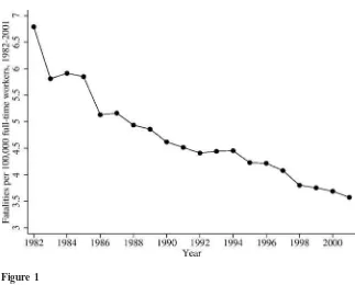
Figure 1
Fatality Rates, 1982–2001
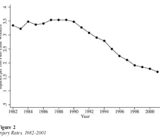
The Bureau of Labor Statistics has recorded injury rates by detailed industry since 1976 as part of their seriesOccupational Injuries and Illnesses in the United States by Industry. They survey about 250,000 firms every year. Over 1982–2001, two variables are consistently recorded—the total injury (and illness) rate and the rate of injuries (and illnesses) resulting in 1 + days away from work. I focus on this latter variable because it is more commonly used in the literature. After merging these data into CPS industries, there are about 180 separate industries. The aggregate injury rate is charted by year in Figure 2. Table A2 shows the ten most dangerous industries and the ten least dangerous industries ranked by the overall injury rate. The correlation between the injury and fatality rates in my data is 0.39.
I report full-sample estimates, but I also split the sample into two smaller time periods. The Census industrial coding system changes in 1992, corresponding to 1991 wages. The classification changes were minor, but “crossing” this 1991 thresh-old requires aggregating a few industries together (Tristao 2006). Consequently, I concentrate on the time periods 1982–90 and 1991–2001.
V. Empirical Strategy
A. Specification
Figure 2
Injury Rates, 1982–2001
Theln(1−τ)variable is used throughout the tax literature (see Gruber and Saez (2002) for one example). The workers’ compensation replacement rate also should impact the relationship between wages and risk since workers in high risk jobs benefit more from a high replacement rate. Because the tax rate directly affects the replacement rate, these variables are not orthogonal and it is important to separately account for the replacement rate. I nonparametrically account for differences between industries through the inclusion of industry-state fixed effects.
Because of nonlinearities in the tax schedule, different industries experience dif-ferent tax changes. Consequently, I must separately account forln(1−τ)to ensure that all comparisons of industries with different risk levels occur for a given tax change. I treat the coefficient onln(1−τ)as a nuisance parameter and do not inter-pret it as the incidence of the income tax. Similarly, I include ln(WC) independently. This strategy can be interpreted as a differences-in-differences framework. I control forln(1−τ)andRand then look at the interaction of the two variables.
The final specification is
′ ′ ′
lnw =γ +α +Xδ +R ρ+β ln (1−τ ) + ln (WC )β
(4) ijkst t sj i t kt 0 ijkst ijkst 1
′ ′ ′ ′
+
[
Rktln (1−τijkst)]
β2+[
Rktln (WCijkst)]
β3+εijkstWCijkst refers to the workers’ compensation after-tax replacement rate (for injuries, deaths, or both), and Xiis a vector of individual-level covariates.Rktrefers to the injury rate, the fatality rate, or both for industry aggregate kat year t. Since there are no national-level workers’ compensation changes and identification ofβ3relies
on state-level changes over time, I include state-industry interactions. More details about this specification are included in the Appendix.
β2 is the coefficient of interest and we expect it to be negative. An increase in the marginal net-of-tax rate should cause the pretax wages of dangerous industries to decrease relative to those of safe industries. We should expectβ3to be negative
as well. A high replacement rate benefits workers in dangerous industries dispro-portionately. In response, pretax wages should decrease relative to the wages of workers in safe industries.
In my instruments, only cross-sectional risk variation is used. Consequently, each industry-state fixed effect is associated with only one risk level in the instrument. These fixed effects account for the cross-sectional correlation between risk and un-observed factors in a completely flexible manner. All standard errors are adjusted for clustering at the industry aggregate level.
B. Heterogeneity in Tax Incidence
The incidence of the tax rate is ∂lnw , holding all other variables constant. While 1
∂
( )
1−τ
changes in the tax rate also directly affect the workers’ compensation replacement rate, the incidence of the tax rate holds this constant (this is suppressed in the notation). This paper focuses on how income taxes distort the relative value of wages and amenities. Tax changes also affect the expected value of wage replacement from the workers’ compensation system. While it is important to explicitly account for the effect of this change in the after-tax replacement rate, the estimate of interest should exclude this channel. Consequently, I hold the after-tax replacement rate constant in the following calculations. In practice, this choice has little effect on the results. I will discuss this issue again briefly when presenting the results.
Evaluating Equation 4, we get
∂lnw ˆ′
=−(β +Rβ)
(5) 0 2
1
∂
( )
ˆ
⎪R
=R 1−τTax incidence focuses on the wage response to tax changes. Identification of β0
is unclear and I have cautioned against interpreting this coefficient as the mean incidence of income taxes. Since this paper looks at heterogeneity in the tax inci-dence, it should not be surprising that this term is differenced out below.
The tax incidence heterogeneity metric is
∂lnw ∂lnw
− =−
[
β +β(Injury)]
+[
β +β (Injury)]
(6) 0 2 h 0 2 l
1 1
∂
( )
⎪
∂( )
⎪
Injury Injury
1−τ h 1−τ l
=β2(Injury−Injury)
l h
As expected, theβ0term drops out. I’ve treated this term as a nuisance parameter because I am not convinced that it can be interpreted solely as the incidence of the marginal tax rate.β2is the only relevant estimate to derive the heterogeneity mea-sure. The calculation using only fatality rates is similar. When both risk rates are included, the following equations are used
′ ′
P(β0+Rβ2≤Ψl) = 0.25, P(β0+Rβ2≤Ψh) = 0.75 The resulting tax incidence heterogeneity metric is
Tax Incidence Heterogeneity =Ψ −Ψ
(7) h l
When both risk rates are used, the percentiles of “riskiness” are implicitly a weighted average of the injury and fatality rates using the regression coefficients as weights. I also present tax heterogeneity metrics which compare the 90th percentile to the 10th percentile. The percentiles defining the dangerous and safe jobs will use the last year of the sample that is used to estimate the coefficients. Because the variation in occupational riskiness is decreasing over time, the early sample coeffi-cients are multiplied by a larger number. It is important to note that there is little reason to think that the tax heterogeneity metric magnitudes will be similar when injury rates or fatality rates are used. These rates may signal certain types of jobs and correlate with different amenities.
C. Description of Instruments
OLS estimation of Specification 4 is problematic since tax rates and replacement rates are functions of the pretax wage. Instead, I employ an instrumental variables (IV) strategy that relies on federal legislative tax changes, state level workers’ com-pensation policy changes, and cross-sectional variation in risk.
A central point of this paper is to understand the consequences of tax changes when amenities do not fully adjust. For this reason, I control separately for the risk level. I also hold risk constant in the instrument when interacting with the tax rate. Holding risk constant has several benefits. First, it ensures that identification only originates from tax schedule changes and not shifts in risk over time. Each risk level in the instruments has a fixed effect associated with it, nonparametrically accounting for omitted variables correlating with risk.
Since the marginal tax rate is a function of an individual’s wage, I must instrument the tax variables. In the spirit of Currie and Gruber (1996a,b), I use a “simulated instrument” by holding a baseline sample constant and allowing the instrument to vary due to federal tax schedule changes only.1
To implement this strategy, I create a baseline sample for each industry and then let tax rates change based on tax schedule changes only. To illustrate this approach, I will detail how I calculate predicted tax rates for each industry in 1985 using federal tax variation only.
1. Create baseline sample (1982 CPS). 2. Inflate incomes to 1985 values.
3. Find tax rate for each person using 1985’s federal tax schedule (and FICA). 4. Average marginal tax rates by industry to get predicted tax rate (τˆjkt). When I focus on my later (1991–2001) sample, my baseline sample is the 1991 CPS. The resulting instrument is ln(1−τˆ
jkt). The variation comes solely from federal tax schedule changes. Industry-state interactions account for fixed wage level dif-ferences.
The workers’ compensation replacement rate also must be instrumented since the replacement rate is a function of the wage. The predicted replacement rate is formed in the exact same way that the predicted tax rates are created, except that the baseline sample also depends on state. The baseline sample is adjusted for inflation for each year and that state-year’s workers’ compensation parameters are applied to each observation. The replacement rates are calculated and averaged by industry and state to getln(WCˆ ). Variation within a state-industry originates solely from state-level
jkst policy changes.
While risk rates change differentially across industries over time in equation (4), I have outlined why it is desirable for exogenous variation in R′ln(1−τ ) to
kt ijkst originate only from changes in the tax schedule. The corresponding instrument in-teracts the log of the predicted net-of-tax rate (as described above) with a risk proxy that does not allow for industry-specific changes over time. An obvious candidate for this risk proxy is the average risk for an industry over the sample period.
The final instruments are: 1. ln(1−τˆjkt)
2. ln(WCˆ jkst) 3. R¯k′×ln(1−τˆjkt) 4. R¯k′×ln(WCˆ jkst)
Figure 3
Average Marginal Tax Rate, 1982–2001
D. Sources of Variation
This paper relies on legislative federal tax changes for identification. The Economic Recovery Tax Act of 1981 (ERTA1981) changed marginal tax rates from 1982 to 1984. The Tax Reform Act of 1986 (TRA1986) is the major tax change during the sample period. TRA1986 drastically reduced the number of income tax brackets and the top federal income tax rate was cut to 28 percent. The Omnibus Budget Rec-onciliation Act of 1990 and 1993 subsequently increased the number of income tax brackets and the top federal income tax rate. In addition, the EITC was significantly expanded during my sample. Figure 3 shows the progression of the average marginal tax rate during the time period 1982–2001.
VI . Results
A. Main Results
OLS results are difficult to interpret and are included in the Appendix (Table A4) for reference. The Appendix also includes the first stage results. Table A5 presents the first stage for the entire sample when both risk rates are included. I report partial F-statistics, which measures the explanatory power of the instruments for each en-dogenous variable independent of the other variables. The first stage is relatively strong for all the variables.
Since most of the tax changes occur in the early part of the sample, the first stage should be much stronger for the 1982–90 sample than the 1991–2001 one. Table A6 shows that this is the case. The partialF-statistics decrease substantially for the later sample. Consequently, we should expect the estimates from the early sample to be much more precise than those from the later one.
The tax incidence heterogeneity numbers compare the elasticity of the wage with respect to the marginal net-of-tax-rate for the 75th (90th) percentile most dangerous industry to the 25th (10th) percentile for the last year of the relevant sample (1990 or 2001) using Equation 7. For reference, Table A7 lists the industries and their risk rates, which are used in these calculations. For example, the full sample uses the 2001 risk distribution. The 25th percentile of the injury rate variable is the Scientific and Controlling Instrument Industry with an injury rate of 0.9 injuries per 100 em-ployees. The 75th percentile is the Engine and Turbines Industry with an injury rate of 2.3. The fatality rates are also included. Table A8 presents the same information for the 90th and 10th percentile.
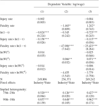
The main results of this paper are shown in Tables 1–3. The reader is encouraged to focus on the tax heterogeneity estimates at the bottom, but the coefficients are also presented. Each table has three columns where each column represents a sepa-rate regression based on which risk sepa-rate is included—injury (Column 1), fatality (Column 2), and both (Column 3). The IV results imply tax incidence heterogeneity of 0.1 to 0.3. This suggests that when the marginal net-of-tax rate decreases 10 percent that the 75th percentile most dangerous job experiences a pretax wage in-crease 1–3 percent larger than the 25th percentile most dangerous job. Comparing the 90th to 10th percentile, the implied heterogeneity is 0.5–0.7. Thus, a 10 percent decrease in the marginal net-of-tax rate causes the wages of the most dangerous jobs to increase by 5–7 percent more than the wages of the safest jobs. Using the mean summary statistics (ignoring variation in initial wages and tax rates between indus-tries), these estimates imply that each percentage point increase in the marginal tax rate increases the pretax wage differential (75th vs. 25th) by $0.07. The 90th vs.10th differential increases by $0.18.
Table 1
Fatality rate 0.660 −0.460
(0.869) (0.880)
Fixed effects Industry*state Industry*state Industry*State Implied Heterogeneity: Significance levels: * 10 percent, ** 5 percent, *** 1 percent. Standard errors in parentheses are clustered by industry aggregate. The “Implied Heterogeneity” results use Equation 7. Covariates include the follow-ing individual characteristics interacted with year dummies: age dummies, gender dummy, race dummies, education dummies.
incidence heterogeneity is now 0.10 to 0.35 using the 75th and 25th percentiles. Using the 90th and 10th, I find incidence heterogeneity of 0.60 to 0.66. While I believe that it is important to directly account for and separately identify the after-tax replacement rate, the final calculations are not meaningfully impacted when they are included.
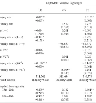
Table 2
IV Results, 1982–90
Dependent Variable: log(wage)
(1) (2) (3)
Injury rate −0.002 −0.004
(0.003) (0.003)
Fixed effects Industry*State Industry*State Industry*State Implied heterogeneity: Significance levels: * 10 percent, ** 5 percent, *** 1 percent. Standard errors in parentheses are clustered by industry aggregate. The “Implied Heterogeneity” results use Equation 7. Covariates include the follow-ing individual characteristics interacted with year dummies: age dummies, gender dummy, race dummies, education dummies.
decrease of 10 percent increases the wages of dangerous jobs by 1–5 percent more than the wages of safe jobs. When comparing the 90th to the 10th percentile jobs, the implied heterogeneity is 0.6 to 1.0.
Table 3
Fixed Effects Industry*State Industry*State Industry*State Implied heterogeneity:
75th–25th 0.479* 0.182 0.461**
(0.249) (0.132) (0.216)
90th–10th 0.902* 1.058 1.482*
(0.468) (0.765) (0.784)
Significance levels: * 10 percent, ** 5 percent, *** 1 percent. Standard errors in parentheses are clustered by industry aggregate. The “Implied Heterogeneity” results use Equation 7. Covariates include the follow-ing individual characteristics interacted with year dummies: age dummies, gender dummy, race dummies, education dummies.
dangerous nature inherent in their jobs are disproportionately harmed. Thus, differ-ential changes in pretax wages imply that income taxes act as taxes on occupational risk at the industry level. The economic implications are potentially profound. If wages are affected, it is likely that other industry-level factors are affected as well. If income taxes act as industry-level taxes on occupational risk, then marginal tax rate increases should shift the marginal cost curve of dangerous industries further than those for safe industries. While beyond the scope of this paper, we should expect to see income taxes differentially affecting the price and output of industries based on their risk level. Such a result implies that the relative production in the economy is not optimal, distorted by income taxation. The tax literature has not studied this possible source of distortion, though the results of this paper suggest that it is a critical consideration for tax policy.
B. Robustness Checks
1. Wage Trends
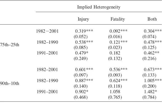
A large literature details the growth of wage inequality during the time period of my sample. A major concern of the analysis in this paper is that wage trends are driving the results. The main results have already provided some evidence that wage trends are not problematic since I use all tax changes as sources of exogenous variation. While TRA1986 did decrease taxes, there are also periods where taxes increased during my sample. The 1991–2001 estimates are more imprecisely mea-sured than the earlier period estimates, but they still suggest very large effects during a period where tax rates increased on average. Thus, legislative tax increases and tax decreases seem to generate similar results, suggesting that secular trends are not driving the results. However, it is useful to account for wage trends more explicitly. In Table 4, I summarize a series of regressions that controls explicitly for initial wages. Each block represents the same regressions seen in the previous tables, but I only report the resulting tax heterogeneity incidence estimates for the sake of simplicity. I compare industries within wage deciles by interacting the year fixed effects with fixed effects based on 1982 (or 1991) wage deciles. These interactions allow low-wage and high-wage industries to experience different year-to-year wage growth. The estimates are consistent with the earlier findings.
im-Table 4
IV Results Controlling for Wage Decile×Year Interactions
Implied Heterogeneity
Injury Fatality Both
75th–25th
1982−2001 0.319*** 0.092*** 0.304***
(0.052) (0.016) (0.074)
1982–1990 0.538*** 0.121*** 0.478***
(0.085) (0.023) (0.125)
1991–2001 0.479* 0.182 0.462**
(0.249) (0.132) (0.216)
90th–10th
1982–2001 0.601*** 0.536*** 0.673***
(0.097) (0.093) (0.133)
1982–1990 0.887*** 0.624*** 1.005***
(0.140) (0.118) (0.200)
1991–2001 0.902* 1.058 1.482*
(0.468) (0.765) (0.784)
Significance levels: * 10 percent, ** 5 percent, *** 1 percent. Standard errors in parentheses are clustered by industry aggregate. The “Implied Heterogeneity” results use Equation 7. Regressions control for wage deciles (based on 1982 or 1991 wage levels) interacted with year fixed effects. Covariates include the following individual characteristics interacted with year dummies: age dummies, gender dummy, race dummies, education dummies.
plicitly comparing industries with similar initial wages is consistent with the ro-bustness of my estimates when initial wages are more explicitly accounted for.
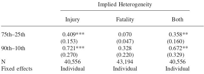
2. Individual level Heterogeneity
Finally, it could be argued that simply accounting for industry-state heterogeneity is inadequate. Instead, we might be concerned that when taxes change, the skill com-position of industries change based on risk. This story suggests that when tax rates change, workers resort themselves across industries. To consider this possibility, I use individual-level panel data to account for individual heterogeneity.
The Panel Survey of Income Dynamics (PSID) records wage and income infor-mation for families for multiple years. I estimate the following specification for the years 1981–96:2
Table 5
Individual-Level Data, 1981–96
Implied Heterogeneity
Injury Fatality Both
75th–25th 0.409*** 0.070 0.358**
(0.153) (0.047) (0.160)
90th–10th 0.721*** 0.328 0.672**
(0.270) (0.220) (0.329)
N 40,556 43,194 40,556
Fixed effects Individual Individual Individual
Significance levels: * 10 percent, ** 5 percent, *** 1 percent. Standard errors in parentheses are clustered by industry aggregate and individual. The “Implied Heterogeneity” results use Equation 7. Covariates include the following individual characteristics interacted with year dummies: age dummies, gender dummy, race dummies, education dummies, tenure at current job, tenure squared.
′ ′ ′
lnw =γ +α +λ +X δ +R ρ+β ln (1−τ ) + ln (WC )β
ijkst t s i it t kt 0 ijkst ijkst 1
(8)
′ ′ ′ ′
+
[
Rktln (1−τijkst)]
β2+[
Rktln (WCijkst)]
β3+εijkstThe strategy is similar. I use tax rates predicted at the industry level in the in-struments. Risk rates are held constant in the instrument and assume that the indi-vidual does not change industries. Similarly, predicted tax rates are assigned assum-ing that the individual does not change industries. Thus, as before, all variation originates from tax schedule changes.
Most people are included in the sample for a significant length of time. It could be argued that an individual fixed effect spanning 16 years is inadequate. Instead, I treat each five-year span for an individual as a separate “person”/fixed effect. In other words, a person in my sample for 1981–90 is treated as two separate people— one for 1981–85 and one for 1986–90.3The standard errors must be appropriately
adjusted and I use the multi-dimensional clustering algorithm suggested by Cameron, Gelbach, and Miller (2011) to account for clustering at the individual level and the levels of the risk measures. Because the injury and fatality rates are provided at different levels, this method implies that I adjust for two-way clustering when one risk rate is included and three-way clustering when both are included.
The PSID sample is much smaller than the CPS so we would expect the estimates to be less precise. There is some evidence of this, but the results in Table 5 are consistent with the CPS results, suggesting that skill and taste heterogeneity are not driving the results presented in this paper. These findings confirm the main results of this paper but are also independently interesting. Hwang, Reed, and Hubbard (1992) presents a model illustrating how skill heterogeneity can bias cross-sectional compensating differential estimates. The results of this paper are likely robust to this
type of critique since identification originates from tax changes, which workers take as given. It is reassuring that including individual fixed effects does not appear to change the estimates.
By controlling for individual heterogeneity, the results in the section suggest that the pretax compensating differential fully adjusts to tax changes. Rosen (1986) pres-ents a model that shows that estimation of compensating differentials by looking at the relationship between an amenity and wages provides the valuation of the mar-ginal worker. This point is relevant to my strategy as well. When tax rates change, the marginal worker might change and pretax wages may not fully adjust due to re-sorting. In terms of interpreting my parameter of interest, this re-sorting is part of the effect of interest since it impacts the observed compensating differential. If workers re-sort to such an extent that pretax compensating differentials adjust less, then this will manifest itself in my result and I will find less heterogeneity in the tax incidence metrics. However, the robustness of the result to individual fixed ef-fects suggests that re-sorting is not impacting the final estimates. Instead, wages appear to fully adjust, keeping the marginal worker relatively constant.
C. Implications for Estimating Compensating Differentials
The results of this paper illustrate that pretax compensating differentials shift with marginal net-of-tax rates. A vast literature studies the relationship between on-the-job risk and wages for the purposes of estimating the value of a statistical life (VSL). The VSL parameter is the implicit tradeoff that individuals make between money and their own probability of dying. This parameter is important for proper cost-benefit analysis of policies which save lives. If a policy costs $3 million per life saved, it is necessary to understand the amount that individuals value those lives saved (or, equivalently, the reduction in their own probability of dying). Equation 1 is the hedonic wage regression typically used in the literature to derive the VSL.
I can calculate how the “observed VSL” (the VSL if pretax wages are used) shifts with taxes. I differentiate Equation 4 with respect to the fatality rate (superscripting all coefficients on fatality variables with F), holding the workers’ compensation variables constant. I evaluate at the mean wage since the specification use the log of the wage and multiply by 200,000 since the fatality rate variable is expressed as fatalities per 200,000 hours. The equation of interest is
F F
Observed VSL =ρ +β ln(1−τ)×w¯×200,000
I calculate how the VSL estimate changes for a one percentage point increase in the marginal tax rate. I perform this calculation at the sample mean marginal tax rate (τ = 0.34):
Observed VSL⎪ −Observed VSL⎪
(9) τ= 0.35 τ= 0.34
F
over $2.6 million. When the Column 3 coefficient estimate is used, the implied increase is about $820,000, though this is insignificant.
These changes in the VSL are relatively large when compared to VSL estimates found in the literature (see Viscusi and Aldy 2003). One concern with VSL estimates generated from studying the cross-sectional relationship between wages and risk is that skill heterogeneity biases the coefficient on risk downward. The Hwang, Reed, and Hubbard (1992) model focuses on skill heterogeneity where high-skilled workers want to be compensated for their skill with a combination of additional safety and wages relative to low-skilled workers. In other words, high-skilled workers sort into safer jobs. The empirical strategy of this paper, however, is likely unaffected by skill heterogeneity. Identification originates from tax changes, which workers take as given and are likely orthogonal to skill level. Consequently, the change in the VSL (estimated above) is unaffected by this critique, while the VSL estimates in the literature are potentially impacted.
The results of this paper produce some meaningful evidence for the VSL and compensating differential literatures. First, cross-sectional wages are a function of risk and other amenities. If workers were not compensated for risk, then taxes would have no effect on the compensating differential. Second, pretax compensating dif-ferentials respond to marginal tax rates and tax rates should be explicitly considered when estimating compensating differentials.
VII. Conclusion
The income tax literature has provided evidence that income taxes distort individuals’ decisions concerning the optimal combination of wages and amenities. Individuals may change occupations to consume different levels of amen-ities or firms may respond in the provision of their amenamen-ities. However, the literature has generally ignored the possibility that some amenities may be, to some extent, defining features of a job and prohibitively costly to change. In these cases, pretax wages must adjust. Thus, tax increases should increase the size of compensating differentials.
I look at the interaction of tax rates and on-the-job safety, finding significantly different wage responses between safe and dangerous jobs. When the marginal net-of-tax rate decreases by 10 percent, the pretax wages of the 75th percentile most dangerous job increase by 1–5 percent more than the pretax wages of the 25th percentile. When comparing the 90th to the 10th percentile, the wages of the dan-gerous job increase by 6–10 percent more. These results suggest that tax increases disproportionately hurt low amenity, high-compensating differential industries and that income taxes act as taxes on low levels of amenities at the industry level. Heterogeneity in the wage response to taxes is economically meaningful and an important component of the total distortion of income taxation.
Data Appendix
A. Fatality Rates
The National Institute for Occupational Safety and Health collected fatality data between 1980 and 20014through the National Traumatic Occupational Fatality
Sur-veillance System (NTOF). The NTOF records fatalities listed as work-related on death certificates, which are coded as externally caused for those that were 16 or older. These fatalities are then categorized by industry. The NTOF typically provides these data at the one-digit SIC level. There are only ten such divisions (including agriculture/forestry/fishing and public administration, both of which are rarely used in this type of analysis), severely limiting the amount of useful variation and reduc-ing any confidence that such a fatality rate accurately describes the true risk expe-rienced by the workers.
By request, I received more detailed fatality data for 49 separate industry cate-gories. To give an example of the importance of this breakdown, the aggregate data set reports one fatality rate for manufacturing. The more detailed data lists fatality rates for 16 different categories within the manufacturing industry. I divide the fa-tality numbers by the total number of hours worked in that industry-year according to the March CPS to arrive at my fatality rate variable.
In the NTOF data, 5.7 percent of fatalities are listed as “Not Classified.” I calculate the percentage of classified fatalities that occur in each industry and make the as-sumption that the unclassified fatalities occurred randomly. Thus, an industry with 2 percent of all classified fatalities in 1985 will be assigned 2 percent of the un-classified fatalities in that year as well. Fatality rates were merged to CIC coding system using the crosswalk provided in Appendix II of Fatal Injuries to Civilian Workers in the United States, 1980–95.
Using death certificates as the only raw data source leads to an undercount of the number of fatalities. This undercount can be estimated by comparisons to the Census of Fatal Occupational Injuries (CFOI). The Bureau of Labor Statistics currently maintains the CFOI which is a highly regarded source for the number of fatalities by industry. However, the CFOI did not begin until 1992. Due to the relatively small federal tax schedule changes between 1992 and 2001, this paper requires fatality data for the pre1992 period.
I compared the CFOI and NTOF rates for 1992–2001. The NTOF recorded 80.6 percent as many fatalities as the CFOI. This number was extremely consistent over time. The annual values ranged from 78.5 percent to 83.3 percent, suggesting that the overall average can be assumed for the pre-1992 period. It is also worth noting that the correlation by NTOF industry-year between NTOF and CFOI fatality rates over this time period is 0.95. This correlation suggests that there is no systematic bias by industry.
B. Injury Rates
able titled “Cases involving days away from work.” The 1982–88 data are catego-rized by the 1977 Standard Industrial Classification system while the 1989–2001 data use the 1987 Standard Industrial Classification system. The data are published at the two-, three-, or four-digit level based on industry. The Census Industrial Clas-sification system used by the CPS, however, is most related to the three-digit SIC level. The four-digit level (reported for manufacturing industries) is too detailed and never used while a few two-digit industries correspond directly to the CIC system. If no injury rate is reported for a given three-digit industry,5 I impute the value
using the injury rate given for its two-digit industry and the other three-digit indus-tries in that two-digit category. The SOII also reports employment data, so I can calculate the injury rate of the “missing industries” within a two-digit category. I use a crosswalk to assign each industry to a CIC category. When one CIC industry corresponds to multiple SIC industries, I average the injury rates, weighted by em-ployment, to the CIC level.
Before 1992, these numbers included fatalities. Since fatalities make up an ex-tremely small percentage of all injuries, it should be acceptable to merge the pre-1992 and pre-1992–2001 data together. Injury rates are reported to one decimal point. Even the injury rates of the highest fatality rate industries would be unaffected by excluding fatality rates at this level. I also show results for an early sub-sample which does not cross this 1992 data change and the estimates appear to be unaf-fected. The BLS simultaneously collects hours data from the surveyed firms and constructs injuries per 200,000 hours (or 100 full-time equivalent workers). C. Sample
My sample includes all workers in the private labor force ages 25–55 that are not self-employed. I exclude all agricultural industries. This leaves me with 757,647 ob-servations. I drop 45,365 observations with allocated wage income, hours worked, or weeks worked. I drop 6,622 observations because they have wages below $2 or above $200 in 2001 dollars. I exclude 19,813 observations because I attribute a workers’ compensation replacement rate (injury or fatality) over 200 percent6to them. Finally,
I only use workers who are listed as the head of the household or the spouse of the head of the household, which excludes 81,490 observations. I am more confident about the tax rates of household heads and their spouses because it is otherwise difficult to determine the tax filing situation. I am left with 604,352 observations.
Table A3 presents summary statistics for the entire sample and subsamples based on overall risk for the entire 1982–2001 period. Wages are listed in 2001 dollars. D. Estimation Details
“Industry aggregate” refers to the level of variation of the risk variable. Each “in-dustry aggregate” includes one or more industries. This is different depending on whether the injury rate is included or the fatality rate is included. The “industry” category refers to the level that the industry fixed effects control for and the level
5. There are several reasons that an injury rate might be missing but, in general, these tend to be very small industries.
of variation for the tax instrument. There are 204 of these industries. To clarify, the value of the risk variables can be the same for several of these industries within a year. The exogenous tax variation, however, will vary for each industry.
I “attach” the injury rate to the temporary total disability replacement rate and the fatality rate to the death benefit replacement rate. I control for the replacement rate(s) related to the risk measures included. I force the coefficient on the death benefit replacement rate to be equal to 0 for single workers with no children. I accomplish this by settingln(WCF ) .
⬅0 ijkst
The covariates are allowed to have different coefficients for each year. The returns to individual characteristics, especially education, are changing over this time period and it is important to account for these changes. I include the following covariates: five-year age group dummies, gender dummies, education dummies, and race dummies.
In practice, I de-mean the risk variables within each year because identification originates from cross-sectional variation in risk. I de-mean the tax and replacement rates by industry because identification originates from industry-specific changes in taxes and replacement rates. De-meaning the input variables is customary with in-teraction terms and does not meaningfully impact the final results here.
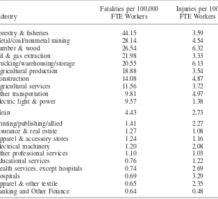
Table A1
Top and Bottom Ten Fatality Rates by Industry, 1982–2001 NTOF Data
Industry
Fatalities per 100,000 FTE Workers
Injuries per 100 FTE Workers
Forestry & fisheries 44.15 3.59
Metal/coal/nonmetal mining 28.14 4.54
Lumber & wood 26.54 6.32
Oil & gas extraction 21.98 3.33
Trucking/warehousing/storage 20.55 6.13
Agricultural production 18.88 3.54
Construction 14.08 4.87
Agricultural services 11.56 3.72
Other transportation 9.81 4.97
Electric light & power 9.57 1.38
Mean 4.43 2.73
Printing/publishing/allied 1.41 2.27
Insurance & real estate 1.27 1.08
Apparel & accessory stores 1.24 1.16
Electrical machinery 1.20 2.08
Other professional services 1.10 1.03
Educational services 0.76 1.22
Health services, except hospitals 0.74 2.69
Hospitals 0.69 3.29
Apparel & other textile 0.65 2.35
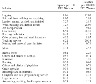
Table A2
Top and Bottom Ten Injury Rates by Industry, 1982–2001 BLS
Industry
Injuries per 100 FTE Workers
Fatalities per 100,000 FTE Workers
Logging 8.66 27.03
Ship and boat building and repairing 8.02 2.99
Leather: tanned, curried, and finished 7.27 5.87
Wood building and mobile homes 7.27 25.07
Air transportation 7.15 9.69
Coal mining 6.58 28.20
Beverage industries 6.44 4.13
Other primary iron and steel industries 6.32 8.97
Trucking service 6.22 20.38
Nursing and personal care facilities 6.18 0.74
Mean 2.73 4.52
Beauty shops 0.62 2.27
Offices and clinics of dentists 0.57 0.74
Insurance 0.55 1.26
Banking 0.54 0.64
Offices and clinics of physicians 0.52 0.74
Credit agencies 0.34 0.62
Brokerage and investments 0.34 0.63
Computer and data programming service 0.34 2.33
Legal services 0.31 1.10
Table A3
Summary Statistics
Entire Sample Lowest Fatality Rate Industries
Mean
Standard
Deviation Mean
Standard Deviation
Wage 17.76 13.24 Wage 18.73 14.54
τ 0.33 0.11 τ 0.34 0.10
Injury rate 2.81 1.96 Injury rate 1.93 1.55
Fatality rate 4.36 5.77 Fatality rate 1.05 0.48
Age 39.23 8.34 Age 39.43 8.31
Percent college 50.02 50.00 Percent college 62.18 48.50 Percent female 45.65 49.81 Percent female 61.57 48.64 Percent white 87.70 32.90 Percent white 87.20 33.41
WCI 0.91 0.23 WCI 0.92 0.24
WCF 0.92 0.26 WCF 0.94 0.26
Middle Fatality Rate Industries Highest Fatality Rate Industries
Mean
Standard
Deviation Mean
Standard Deviation
Wage 16.59 12.54 Wage 17.92 11.83
τ 0.32 0.12 τ 0.32 0.11
Injury rate 2.62 1.53 Injury rate 4.45 2.07
Fatality rate 2.85 0.87 Fatality rate 11.80 7.51
Age 39.03 8.40 Age 39.21 8.30
Percent college 45.87 49.83 Percent college 36.58 48.17 Percent female 43.13 49.53 Percent female 23.83 42.61 Percent white 87.00 33.63 Percent white 89.32 30.89
WCI 0.91 0.23 WCI 0.88 0.22
Table A4
OLS Results, 1982–2001
Dependent Variable: log(wage)
(1) (2) (3)
Injury rate 0.003
(0.002)
0.003 (0.002)
Fatality rate 1.686
(0.690)
0.507 (0.987)
ln(1−τ) −1.791*** −1.697*** −1.780***
(0.015) (0.021) (0.017)
Injury rate×ln(1−τ) −0.018** −0.031***
(0.007) (0.008)
Fatality rate×ln(1−τ) 1.085 8.195***
(2.286) (2.468)
ln(WCI) −0.953*** −0.753***
(0.012) (0.013)
ln(WCF) −0.779*** −0.239***
(0.011) (0.011)
Injury rate×ln(WCI) −0.016*** −0.016**
(0.006) (0.006)
Fatality rate×ln(WCF) −1.222 0.479
(2.464) (2.438)
N 594,119 598,438 591,920
Fixed Effects Industry*State Industry*State Industry*State Implied heterogeneity:
75th–25th 0.025** −0.002 0.039***
(0.010) (0.004) (0.011)
90th–10th 0.047** −0.012 0.066***
(0.019) (0.025) (0.022)
Powell
N 591,920 591,920 591,920 591,920 591,920 591,920 591,920
PartialF-Statistic 101.49 285.50 100.21 568.63 61.44 246.24 164.56
Table A6
PartialF-Statistics by Sample
1982–2001 1982–90 1991–2001
ln(1−τ) 101.49 117.98 5.98
Injury×ln(1−τ) 285.50 517.33 62.68
Fatal×ln(1−τ) 100.21 165.57 4.48
ln(WCI) 568.63 583.51 347.42
ln(WCF) 61.44 93.60 115.89
Injury×ln(WCI) 246.24 286.66 114.96
Fatal×ln(WCF) 164.46 236.72 41.45
N 591,920 249,242 310,579
Each column reports the partialF-statistics for each variable for that sample. Covariates include Indus-try*State dummy variables and the following individual characteristics interacted with year dummies: age dummies, gender dummy, race dummies, education dummies.
Table A7
Injury and Fatality Rates for Tax Incidence Heterogeneity Calculation (75th–25th)
Injury Rates
75th Percentile 25th Percentile
2001 Engines and Turbines 2.3 per 100
Scientific and Controlling Instrument 0.9 per 100 1990 Crude petroleum & natural gas
extraction
Colleges and universities 1.7 per 100 5.0 per 100
Fatality Rates
75th Percentile 25th Percentile
2001 Motor Vehicles/Auto Supply Dealer Other Professional
2.7 per 100,000 0.8 per 100,000
1990 Motor vehicles/auto supply dealer Insurance and real estate
Table A8
Injury and Fatality Rates for Tax Incidence Heterogeneity Calculation (90th–10th)
Injury Rates
90th Percentile 10th Percentile
2001 Construction Banking
3.0 per 100 0.4 per 100
1990 Construction Other health services
6.2 per 100 0.8 per 100
Fatality Rates
90th Percentile 10th Percentile
2001 Construction Apparel & accessory store
11.5 per 100,000 0.5 per 100,000
1990 Construction Banking
14.5 per 100,000 0.7 per 100,000
References
Albouy, David. 2009. “The Unequal Geographic Burden of Federal Taxation.”Journal of Political Economy117(4):635–67.
Cameron, A. Colin, Jonah Gelbach, and Douglas Miller. 2011. “Robust Inference with Mul-tiway Clustering.”Journal of Business and Economic Statistics29(2):238–49.
Currie, Janet, and Jonathan Gruber. 1996a. “Saving Babies: The Efficacy and Cost of Re-cent Changes in the Medicaid Eligibility of Pregnant Women.”Journal of Political Econ-omy104(6):1263–96.
———. 1996b. “Health Insurance Eligibility, Utilization of Medical Care, and Child Health.”Quarterly Journal of Economics111(2):431–66.
Feenberg, Daniel, and Elisabeth Coutts. 1993. “An Introduction to the TAXSIM Model.”
Journal of Policy Analysis and Management12(1):189–94.
Gruber, Jonathan, and Michael Lettau. 2004. “How Elastic is the Firm’s Demand for Health Insurance.”Journal of Public Economics88(7–8):1273–93.
Gruber, Jonathan, and Emmanuel Saez. 2002. “The Elasticity of Taxable Income: Evidence and Implications.”Journal of Public Economics84(1):1–32.
Hamermesh, Daniel. 1999. “Changing Inequality in Markets for Workplace Amenities.”
Quarterly Journal of Economics114(4):1085–123.
Hwang, Hae-shin, W. Robert Reed, and Carlton Hubbard. 1992. “Compensating Wage Dif-ferentials and Unobserved Productivity.”Journal of Political Economy100(4):835–58. Kniesner, Thomas, and John Leeth. 2010. “Hedonic Wage Equilibrium: Theory, Evidence
Kubik, Jeffrey. 2004. “The Incidence of Personal Income Taxation: Evidence from the Tax Reform Act of 1986.”Journal of Public Economics88(7–8):1567–88.
Leigh, Andrew. 2010. “Who Benefits from the Earned Income Tax Credit? Incidence Among Recipients, Coworkers and Firms.”B.E. Journal of Economic Analysis & Policy
10(1):45.
Marsh, Suzanne, and Larry Layne. 2001. “Fatal Injuries to Civilian Workers in the United States, 1980–1995. Department of Health and Human Services. Publication No. 2001– 129.
Powell, David, and Hui Shan. 2012. “Income Taxes, Compensating Differentials, and Occu-pational Choice: How Taxes Distort the Wage-Amenity Decision.American Economic Journal: Economic Policy4(1).
Rosen, Sherwin. 1986. “The Theory of Equalizing Differences.”Handbook of Labor Eco-nomics1:641–692.
Smith, Adam. 1947.An Inquiry into the Nature and Causes of the Wealth of Nations. Mod-ern Library Edition.
Tristao, Ignez. 2006. “Matching Industry Codes Over Time and Across Classification Sys-tems: A Crosswalk for the Standard Industrial Classification to the Census Industry Clas-sification System.” University of Maryland. Unpublished.