Manajemen | Fakultas Ekonomi Universitas Maritim Raja Ali Haji 073500103288619359

Full Terms & Conditions of access and use can be found at

http://www.tandfonline.com/action/journalInformation?journalCode=ubes20

Download by: [Universitas Maritim Raja Ali Haji] Date: 13 January 2016, At: 00:19

Journal of Business & Economic Statistics

ISSN: 0735-0015 (Print) 1537-2707 (Online) Journal homepage: http://www.tandfonline.com/loi/ubes20

Moment and Memory Properties of Linear

Conditional Heteroscedasticity Models, and a New

Model

James Davidson

To cite this article: James Davidson (2004) Moment and Memory Properties of Linear

Conditional Heteroscedasticity Models, and a New Model, Journal of Business & Economic Statistics, 22:1, 16-29, DOI: 10.1198/073500103288619359

To link to this article: http://dx.doi.org/10.1198/073500103288619359

Published online: 01 Jan 2012.

Submit your article to this journal

Article views: 143

View related articles

Moment and Memory Properties of Linear

Conditional Heteroscedasticity Models,

and a New Model

James D

AVIDSON

Cardiff Business School, Cardiff CF10 3EU, U.K. (davidsonje@cardiff.ac.uk)

This article analyses the statistical properties of that general class of conditional heteroscedasticity models in which the conditional variance is a linear function of squared lags of the process. GARCH, IGARCH, FIGARCH, and a newly proposed generalization, the HYGARCH model, belong to this class. Conditions are derived for the existence of second and fourth moments, and for the limited memory condition of near-epoch dependence. The HYGARCH model is applied to 10 daily dollar exchange rates, and also to data for Asian exchange rates over the 1997 crisis period. In the latter case, the model exhibits notable stability across the pre-crisis and post-crisis periods.

KEY WORDS: ARCH(inŽnity); FIGARCH; Hyperbolic lag; Near-epoch dependence; Exchange rate.

1. INTRODUCTION

Many variants of Engle’s (1982) ARCH model of conditional volatility have been proposed, including GARCH (Bollerslev 1986), IGARCH (Engle and Bollerslev 1986), and FIGARCH (Baillie, Bollerslev, and Mikkelsen 1996; Ding and Granger 1996). All of these models, and many other cases that might be devised, fall into the class in which the conditional variance at timetis an inŽnite moving average of the squared realizations of the series up to timet_¡1:Formally, let

utD¾tet; (1)

where¾t>0,et»iid.0;1/, and

¾_t2_D!_C

1

X

i_D1

µiu2t_¡i; µi¸0 for alli; (2)

where µi are lag coefŽcients typically depending on a small

number of underlying parameters. By adding an error term, vtDu2t ¡¾t2, to both sides, (2) can be viewed as an AR(1) in

the squared series, and hence is commonly called an ARCH(₁) model.

In the well-known case of the GARCH(1;1) model,

¾_t2_D° _C®1u2_t¡1C¯1¾_t2_¡1 (3)

solves to give (2) with µi D®1¯₁i¡1 for i¸1, and !D° =

.1_¡¯1/. The stationarity condition is well known to be®1C

¯1<1, which is equivalent to

1

X

i_D1

µi<1: (4)

The IGARCH case is the variant in which ®1C¯1D1, and

hence the sum of the lag coefŽcients is also unity, where the

µi’s form a convergent geometric series.

Generalizing to the higher-order cases, let±.L/_D1_¡±1L¡

¢ ¢ ¢¡±pL

p

and¯ .L/_D1_¡¯1L¡ ¢ ¢ ¢¡¯pL

p

denote polynomials in the lag operator. The GARCH(p;q) model can be expressed in the “ARMA-in-squares” form,

±.L/u2_{t D}°_C¯.L/vt; (5)

wherevtDu2t ¡¾t2D.e2t ¡1/¾t2, as well as in the more

con-ventional representation,

¯ .L/¾_t2_D° _C¡¯.L/_¡±.L/¢u2_t; (6) so that®1D±1¡¯1in the notation of (3). The model is

re-arranged into the form of (2) as

¾_t2_D ° ¯ .1/C

³

1_¡ ±.L/

¯ .L/

´

u2_{t D}!_Cµ .L/u2_t; (7)

whereµ .L/_DP1

iD1µiLi. Note thatµ0D0 by construction here.

The general IGARCH(p;q) can be represented by (7) subject to the constraint±.1/_D0, such that the lag coefŽcients sum to unity. More explicitly, it might be written in the form

µ .L/_D1_¡ ±.L/

¯ .L/.1¡L/; (8)

where ±.L/is deŽned appropriately. However, it is important to note the fact that there is no explicit requirement for the roots of ±.L/to be stable. Nelson (1990) showed that in the GARCH(1;1) case,±1>1 is compatible with strict stationarity,

but not with covariance stationarity. See Section 3.2 for more on this case.

The FIGARCH(p;d;q) model replaces the simple difference in (8) with a fractional difference, such that

µ .L/_D1_¡±.L/

¯ .L/.1¡L/

d ₍₉₎

for 0<d<1. The FIGARCH is a case where the lag coef-Žcients decline hyperbolically, rather than geometrically, to 0, and it is on these cases that this article focuses. This form has been used in a number of recent works to model Žnancial time series (see, e.g., Baillie et al. 1996; Beltratti and Morana 1999; Baillie, Cecen, and Han 2000; Baillie and Osterberg 2000; Brunetti and Gilbert 2000). As is well known,

.1_¡L/d_D1_¡ 1

X

iD1

ajLj; (10)

© 2004 American Statistical Association Journal of Business & Economic Statistics January 2004, Vol. 22, No. 1 DOI 10.1198/073500103288619359

16

where

ajD

d0. j_¡d/

0.1_¡d/0. j_C1/DO.j

¡1_¡d_{/: (11)}

This article focuses attention on these linear-in-the-squares models, in contrast to such cases as EGARCH (Nelson 1991), where the logarithm of the conditional variance is modeled. As will become clear in the sequel, the moment and mem-ory properties of the latter type of model must be analyzed in a different way. An important related study by Giraitis, Kokoszka, and Leipus (2000) (henceforth GKL) studied the squared process _fu2_tg itself, and some of the results here can be seen as complementary to theirs. The focus here is on the process_futg itself, primarily because, as discussed in

Sec-tion 3.1, the results have a direct applicaSec-tion to the asymptotic analysis of conditionally heteroscedastic series. The existence of moments and also the conditions for limited memory, char-acterized here as near-epoch dependence on the independent processet, are considered.

Section 2 considers the conditions for second-order station-arity, and also sufŽcient conditions for fourth-order stationarity. Section 3.1 addresses the near-epoch dependence question, and Section 3.2 proves a modiŽed short-memory property for the class of non-wide sense stationary cases, such as the IGARCH, for which the variance does not exist, subject to strict stationar-ity. Section 4 further discusses some features of the IGARCH and FIGARCH models. Some puzzles and paradoxes that have been discussed in the literature are resolved by noting that in-dependent parameter restrictions control the existence of mo-ments and the memory of the volatility process. IGARCH and FIGARCH models have been described in the literature as “long memory,” by an implicit analogy with the integrated or fractionally integrated linear model of the conditional mean. However, a conclusion that is emphasized is that such analo-gies are generally misleading. It turns out that ARCH(₁) mod-els cannot exhibit long memory by the usual criteria. Both the sequence of lag coefŽcients and the autocorrelations of the squared process when these are deŽned must be summable, to avoid nonstationary (explosive) solutions.

Section 5 introduces a new model, the HYGARCH, gener-alizing the FIGARCH, that can be covariance stationary while exhibiting hyperbolic memory. Section 6 reports some applica-tions of the latter model. Section 6.1 applies it to some famil-iar series, and Section 6.2 considers Asian exchange rate data covering the 1997–1998 crisis period. Section 7 concludes the article.

2. MOMENT PROPERTIES

Volatility models of the ARCH(₁) class have two salient features, which in this article will be referred to as, respec-tively, the amplitude and the memory. The amplitude deter-mines how large the variations in the conditional variance can be, and hence the order of existing moments, whereas the memory determines how long shocks to the volatility take to dissipate. The amplitude is measured by

S_D

1

X

i_D1

µi: (12)

Regarding the phenomenon of (limited) memory, two cases are recognized. Hyperbolic memory is measured by the parame-ter±, such that

µiDO.i¡1¡±/: (13)

Geometric memory is measured by the parameter½, where

µiDO.½¡i/: (14)

Note that the “length” of memory variesinverselywith these parameters. In the geometric-decay GARCH(1;1) model, for example,S_D®1=.1¡¯1/, and½D1=¯1. Although in the case

where½ >1, the hyperbolic memory assumes the value_C1, it is more realistic to recognize that these represent two different modes of memory decay in which the low-order lags of one can dominate those of the other in either case. What is true is that the hyperbolic lags must always dominate the geometric by takingilarge enough.

The condition

S<1 (15)

is generally necessary and sufŽcient for covariance stationarity. To see this, writeMpDEupt, assumed to not depend ont. Then

for the casep_D2, by the law of iterated expectations,

E¾_t2_DEu2_{t D}!_C

1

X

iD1

µiEu2t¡i; (16)

with the stationary solution

M2D

!

1_¡S: (17)

Next, consider the fourth moment. Letting¹4DEe4t, note

thatEu4_{t D}¹4E¾t4, where

E¾_t4_D!2_C2!

1

X

i_D1

µiEu2t¡iC 1

X

i_D1 1

X

j_D1

µiµjEu2t¡iu2t¡j: (18)

Even assuming that these expectations do not depend ont, to solve the equality in (18) exactly is intractable. However, the Cauchy–Schwarz inequality will imply Eu2_t¡iu2_{t¡j ·}M4, and

hence

M4·¹4

³

!2_C2!

2_S

1_¡S CS

2_M

4

´

(19)

or, equivalently,

M4·

¹4!2.1CS/

.1_¡S/.1_¡¹4S2/

: (20)

The condition

¹4S2<1 (21)

is therefore sufŽcient, although not necessary, for the exis-tence ofM4and fourth-order stationarity. Conditions equivalent

to (15) and (21) were also derived by GKL, who considered the conditions for a weakly stationary solution of the processu2_t:

It is of interest to evaluate the bound in (21) for a case where the exact necessary condition for fourth-order stationarity is known. The GARCH(1;1) in (3) hasS_D®1=.1¡¯1/.

forward manipulations show that

M4D

¹4°2.1¡¯1/2.1C®1C¯1/

.1_¡®1¡¯1/.1¡¹4®2₁¡2®1¯1¡¯₁2/

; (22)

subject to second-order stationarity and satisfaction of the extra inequality

®2₁¹4<1¡2®1¯1¡¯12: (23)

This result may be derived as a special case of that given by Davidson (2002) for the GARCH(p;p). (For another version of the general formula, see He and Teräsvirta 1999, and for the Gaussian case see Karonasos 1999.) Note that (21) can be re-arranged as

®2₁¹4<1¡2¯1C¯12: (24)

The majorants of (23) and (24) differ by 2¯1.1¡®1¡¯1/,

and therefore the latter condition binds as this quantity ap-proaches 0. In this example, the sufŽcient condition imposes too tough a constraint on the kurtosis of the shocks when the variance is not too large. However, note that the two conditions are identical in the ARCH(1) model, when ¯1D0. They are

also similar in the region where the second-order stationarity condition is tending to bind, and eventually coincide, although note that to fall in this region requires that¹4be close to 1.

3. MEMORY PROPERTIES 3.1 Near-Epoch Dependence

There are a number of ways to measure the memory of a process, some speciŽc to the model structure (e.g., the rate of decay of the weights of a linear process) and some model-independent,(e.g., the various mixing conditions). The correlo-gram measures only one facet of the memory of a nonlinear process, although the correlogram of the squared process supplies additional information relevant to conditional het-eroscedasticity in particular. The analysis of GKL is germane to this case. The motivation for studying memory properties is sometimes related to forecastability at long range, but more often concern focuses on checking the validity of applying av-eraging operations to a time series, to estimate parameters and undertake statistical inference. As is well known, the validity of the central limit theorem (CLT) and law of large numbers depends critically on remote parts of a sequence being indepen-dent of each other, in an appropriate sense.

Uncorrelatedness at long range is not a sufŽcient condition to validate the CLT, and although the mixing property is often invoked, it is difŽcult to verify. However, the property of near-epoch dependence on a mixing process can sufŽce. This is the property that the error in the best predictor of the process, based on only the “near epoch” of an underlying mixing process, is sufŽciently small. Thus, lettingF_st_D¾ .es; : : : ;et/be the sigma

Želd generated by the collection _fej;s·j·tg, a process ut

is said to be Lp-near-epoch–dependent (Lp-NED) on fetg of

size_¡¸0if

kut¡E.utjFtt_¡Cmm/kp·dtm¡¸ (25)

for¸ > ¸0. In the general deŽnition,dt is a sequence of

posi-tive constants, but subject to stationarity, as here, one may sim-ply write dtDd<1 (see Davidson 1994, chap. 17, among

other references, for additional details). Ifm¡¸can be replaced

with½¡m in (25), then the process will be said to be geomet-rically NED. There is no accepted “size” terminology associ-ated with this case, but obviously one can speak of “geometric size½” in a consistent manner, if it is convenient to do so.

In the present application,the process_fetgwill be taken as the

driving process in (1). Because this is not merely mixing but iid, by assumption, the condition in (25) alone constrains the mem-ory of the process. The application of this approach to a range of nonlinear processes, including GARCH processes, has been studied earlier (Davidson 2002). Following the same approach, the present work now derives conditions forut deŽned by (1)

plus (2) to be L1 orL2-NED onfetg. In the following result

for the hyperbolic memory case, the model is formalized just to the extent of specifying the lag coefŽcients to be bounded by a regularly varying function. This strengthens the summability requirement, but only slightly.

Theorem 1. a. If 0_·µi·Ci¡1¡± fori¸1, forC>0, and

± > ¸0¸0 andS<1, thenutisL1-NED onfetg, of size¡¸0.

b. If in additionS< ¹¡₄1=2, thenutisL2-NED of size¡¸0:

The proof, given in the Appendix, follows GKL in working with a Volterra-type series expansion of the process to construct the near-epoch–based predictor and bound its residual.

GKL have shown that the process_fu2_tghas absolutely sum-mable autocovariances,subject only to the conditionS< ¹¡₄1=2. No separate constraint on the rate of convergence of the lag coefŽcients is speciŽed in their result, although summability obviously requires± >0, so that their conditions match those forL2-NED of size 0. These authors also proved a CLT for the

process_fu2_{t ¡}Eu2_tg subject only to the same condition on the sum. The CLT forL2-NED processes of De Jong (1997), such

as might be applied to futg using the present result, calls for

¸0D1=2. This provides what to the author’s knowledge is the

best CLT currently available for ARCH(₁) processes. Extend-ing the result of GKL to the same case is not trivial, because the reverse mapping fromu2_t tout is not single valued, but there is

the strong suggestion that still-sharper conditions for the CLT for_futgmight be obtainable by exploiting the properties of the

process more directly. Essentially, even with decay rates slower than_¡1=2, the restriction on the sum of the coefŽcients may force them to be individually so small that negligibility argu-ments can be applied to the tail of the lag distribution. This is an interesting direction for further research.

The following is the corresponding result for the geometric memory case.

Theorem 2. a. If 0_·µi·C½¡i fori¸1, with 0<C< ½

and½ >1 andS<1, thenutis geometricallyL1-NED onfetg.

b. If in addition,C< ½¹¡₄1=2andS< ¹¡₄1=2, thenut is

geo-metricallyL2-NED:

The GARCH(p;q) is the leading example of the geometric case, and this result may be compared with proposition 2.3 of Davidson (2002). Note that becauseµ1·C½¡1 and

necessar-ilyµ1<S, the sufŽcient restrictions on C in Theorem 2 are

minimal, in view of the restrictions onS:In effect, they forbid isolated inuential lags of higher order. Inspection of the proof show that they could be relaxed, at the cost of more complex or specialized conditions. The important point to note about both of these results is that the existence of second (fourth) moments is necessary and nearly sufŽcient for theL1-NED (L2-NED)

property.

3.2 The Nonstationary Geometric Lag Case

Nelson (1990) gave an insightful analysis of persistence (memory) in the GARCH(1;1) model. The key condition that he derived for limited persistence (what he would call “nonper-sistence”) is

Eln.¯1C®1e2_t/ <0; (26)

and the Jensen inequality easily shows that the condition

®1<1¡¯1is sufŽcient for (26). This condition is necessary

and sufŽcient for the process to be strictly stationary and er-godic (Nelson 1990, thm. 2).

Necessary conditions for strict stationarity of the GARCH(1;1) depend on the distribution ofet, and are shown

for the standard Gaussian case in Nelson’s (1990) Žgure 8.1 as a nonlinear trade-off between the values of®1and¯1:In that

case, note that strict stationarity is compatible with nonexis-tence of second moments, and Nelson’s Žgure shows that, for example,®1>3 is permitted when¯1is close enough to 0.

The NED measure of memory is unavailable without Žrst moments, but an alternative is provided by the notion of L0-approximability due to Pötscher and Prucha (1991) (see

also Davidson 1994, chap. 17.4). This is the condition that there exists a locally measurable (Žnite-lag) approximation to ut, which is a uniform mixing process, given thatet is

in-dependent (e.g., Davidson 1994, thm 14.1). Let hm_t denote a FtCm

t¡m-measurable approximation function, depending only

onet¡m; : : : ;etin the present case. Then deŽnehmt to be a

geo-metricallyL0-approximator of¾t2if

P._j¾_t2_¡hm_{t j}>dt±/DO.½¡m/ (27)

for ½ >1 and all ± >0, where, subject to stationarity as as-sumed here, we may set dtD1. The following result can now

be obtained.

Theorem 3. Let ut be a strictly stationary process, and

0·µi·C½¡i fori¸1 with½ >1. In either of the following

cases,¾_t2is geometricallyL0-approximable:

a. C< ½.

b. C< ½ .½_¡1/and log.C1C"=.½1C"_¡1// < ³ for some

" >0, where³ _DE._¡loge2_t/:

Note thatS_·C=.½ _¡1/, and hence the restriction onCin part (b), as well as that in part (a), implies thatS< ½. However, Scan substantially exceed 1 in either case, if½is large enough. In addition, inspection of the proof shows that these conditions are only sufŽcient, and theL0-approximabilityproperty still

ob-tains in numerous cases where (a) and (b) are violated, but are awkward to state compactly.

Taking the GARCH(1;1) as an example, we Žnd ½_D¯₁¡1

andC_D®1=¯1, so the condition to be satisŽed in (a) is®1<1,

and that in (b) is ®1<1=¯1¡1. It is an interesting

ques-tion to relate the condiques-tions of the theorem to condiques-tions for strict stationarity such as (26). Kazakevicius and Leipus (2002,Ï thm. 2.3) have shown that log.C=.½ _¡1// < ³ is a necessary condition for strict stationarity, although not sufŽcient, because in the case of the GARCH(1;1) this is actually a weaker con-dition than (26). WhenC< ½, thenC½¡j<1 for allj_¸1, and also note thatC1C"_=.½1_C"_{¡1/ <C=.½ ¡1/for" >0, which}

guarantees that the second condition in (b) holds in a stationary

process. But, whenC_¸½, condition (b) can evidently fail in a stationary process. Note that although the present proof es-tablishes independence of initial conditions, it makes use of the stationarity assumption and thus cannot provide a proof of sta-tionarity as such.

The conceptual importance of this result is chiey to show the way in which short memory is a feature of the strictly stationary case, whether moments exist or not. From a more practical viewpoint, though, the property might be used in con-junction with mixing limit theorems to show that, for example, a law of large numbers applies to integrable transformations of the process, such as truncations. (See Pötscher and Prucha 1991 and Davidson 1994 for more details of this approach.)

4. THE IGARCH AND FIGARCH MODELS

The interesting feature of ARCH(₁) models revealed by the foregoing analysis is that the rate of convergence of the lag coefŽcients to 0 is irrelevant to the covariance stationar-ity property, provided that these are summable. The key con-straint is the relationship of their sum to unity. When this is equal to or exceeds unity, no second moments exist regard-less of the memory of the process. The familiar example is the IGARCH(1;1) model, which, according to Theorem 3, is geo-metricallyL0-approximable, or in other words, short memory.

This appears to be paradoxical, because the IGARCH model is often spoken of in the literature as a “long memory” model, the volatility counterpart of the unit root model of levels. Con-sider thek-step-ahead “volatility forecast” from the model rep-resented by

¾_t2_D °

1_¡¯1C

.1_¡¯1/ 1

X

j_D1

¯₁j¡1u2_t¡j

D°_C.1_¡¯1/u2t_¡1C¯1¾t2_¡1: (28)

Applying the law of iterated expectations would appear to yield the solution

Etu2_tCkDk° Cu2t; (29)

which, although diverging, remains dependent on current con-ditions even at long range. Thus it appears thatu2_t fulŽls the condition for long memory proposed by Granger and Terasvirta (1993, p. 49)—that is, to be forecastable in mean at long range. But this is a paradox, because¾_t2clearly depends only on the re-cent past. Theorem 3a shows that¾_t2can be reconstructed from the shock history,_fet_¡1;et_¡2; : : : ;et_¡mg, with an error that

van-ishes at an exponential rate asmincreases, so clearly it cannot be forecast at long range.

Ding and Granger (1996) discussed this apparent paradox of memory by considering the extreme case in which¯1D0 and

° _D0;so that (29) reduces toEtu2_tCkDu2t. This model can be

written in the form

utDetjut¡1j: (30)

Although a succession of larger-than-average independent shocks (et’s) may produce very large deviations of the observed

process, such that their variance is inŽnite, the et’s are still

drawn independently from a distribution centered on 0. Note

how a single “small deviation” ofet (having the highest

prob-ability density of occurrence, in general) kills a “run” of high volatility instantly. That the probability of such an event occur-ring in (30) converges rapidly to 1, is the essential message of Theorem 3. Nelson (1990) showed that this particular process converges to 0 in a Žnite number of steps, with probability 1.

The present results allow consideration of a still more ex-treme case, that of ¾_t2_D®u2_t¡1 for® >1. Some substitutions yield

¾_t2_D®e2_t¡1¾_t2_{¡1D ¢ ¢ ¢ D}®me_t2_¡1e2_{t¡2¢ ¢ ¢}e2_t¡m¾_t2_¡m: (31)

Noting that in this case the sum of the lag coefŽcents is®(this can be treated as the limiting case as ½_{! 1} andC_D®½), applying Theorem 3b shows that the steady state solution is

¾_t2_D0 whenever log® <_¡Eloge2_t. In this case, the right side of (31) converges to 0 in probability (in fact, with probability 1) asm_Dtincreases, starting from any Žxed¾₀2>0.

The straightforward solution to the paradox presented by these cases is that although¾_t2in (28) or (31) is a natural in-dicator of conditional volatility, depending on the near epoch, it isnotthe conditional variance. Because the unconditionalvari-ance does not exist in these cases, the conditional variunconditionalvari-ance is not a well-deŽned random variable. Note that the application of the law of iterated expectations is not valid here, so (29) has no meaningful interpretation. These examples highlight the im-portant distinction to be maintained between the moment and memory properties of a sequence.

The FIGARCH model deŽned by (9) is a generalization of the IGARCH, of particular interest because this is the one application to date using hyperbolic lag weights. Note that

P1

iD1ajD1 in (10) for any value ofd, and this therefore

be-longs to the same “knife-edge-nonstationary” class represented by the IGARCH, with which it coincides ford_D1. However, note the interesting and counterintuitive fact that the length of the memory of this process is increasingas d approaches 0. [Note the error in Baillie et al. 1996, p. 11, line 6, where the lag coefŽcients are said to be of O.kd¡1/. This should read O.k¡d¡1_{/.] This is, of course, the opposite of the role ofdin the}

fractionally integrated process in levels. Note that whend_D1, then a1D1, andaiD0 for i>1: In this particular case, of

amplitudeS_D1, the memory [measured by_¡±in (13)] is dis-continuous, jumping to_¡1at the point where it attains_¡1.

At the other extreme, asdapproaches 0, the lag weights are approaching nonsummability. However, again because of the restrictionS_D1;the individualai’s are all approaching 0. The

limiting cased_D0 is actually another short-memory case, in this case the stable GARCH rather than the IGARCH repre-sented byd_D1:Atd_D0, the memory jumps from 0 to_¡1, and the amplitude is also discontinuous at this point, jumping from a Žxed value of 1 to some value strictly below 1. The char-acterization of the FIGARCH model as an intermediate case between the stable GARCH and the IGARCH, just as the I(d) process in levels is intermediate between I(0) and I(1) is there-fore misleading. In fact, it has more memory than either of these models, but behaves oddly owing to the rather arbitrary restric-tion of holding the amplitude to 1 (the knife-edge value) while the memory increases.

The term “long memory” has been applied to the FIGARCH model by several authors, for understandable reasons, but our

discussion has made clear that the analogy with models of the conditional mean is also misleading in this respect. To illus-trate the dangers of taking the “AR-in-squares” characterization of these models too literally, consider the simplest FIGARCH model,

¾_t2_D!_C¡1_¡.1_¡L/d¢u2_t; (32) rearranged as

.1_¡L/du2_{t D}!_Cvt; (33)

withvtD.e2t ¡1/¾t2as earlier. This equation might appear to

representu2_t as a classic fractionally integrated process. How-ever, just as the temptation to write E.vt/D0 must be

re-sisted, in the absence of second moments, so it is important to not confuse this formal representation (in which vt does

not represent a forcing process and is serially dependent) with the data-generation process. Indeed, were one to replace vt

in (33) by (say) an independent disturbance with mean of 0 for t>0, and by 0 fort_·0, then one would actually obtain a non-stationarytrendingprocess with expected value!tdfort>0 (see Granger 2002). This clearly contradicts what is known about the actual characteristics of theu2_t process.

As remarked earlier, GKL showed that whenever fourth mo-ments exist, the autocovariances of the squared process are always summable. Kazakevicius and Leipus (2002) furtherÏ showed that summability of the ARCH(₁) lag weights is a nec-essary condition for stationarity. Long memory in mean, char-acterized by nonsummable autocovariances, does not appear to have a well-deŽned counterpart in the ARCH(₁) framework, whether or not moments exist, because in any such cases the processes must diverge rapidly. The term “hyperbolic memory” is therefore preferable to distinguish FIGARCH from the geo-metric memory cases such as GARCH and IGARCH.

5. THE HYGARCH MODEL

The unexpected behavior of the FIGARCH model may be due less to any inherent paradoxes than to the fact that the unit-amplitude restriction, appropriate to a model of levels, has been transplanted into a model of volatility. In a more general frame-work, there are good reasons to embed it in a class of models in which such restrictions can be tested, and also to adhere to the approach of modeling amplitude and memory as separate phenomena, just as is done in the ordinary GARCH model.

In view of these considerations a new model is here pro-posed, the “hyperbolic GARCH,” or HYGARCH model. Con-sider, for comparability with the previous cases, the form

µ .L/_D1_¡ ±.L/

¯.L/

¡

1_C®..1_¡L/d_¡1/¢

; (34)

where®_¸0,d_¸0. Note that, provided thatd>0,

S_D1_¡ ±.1/

¯.1/.1¡®/: (35)

The FIGARCH and stable GARCH cases correspond to®_D1 and®_D0, respectively, and in principle, the hypothesis of ei-ther of these two pure cases might be tested. However, in the latter case the parameterdis unidentiŽed, which poses a

known problem for constructing hypothesis tests. Therefore, also note that whend_D1, (34) reduces to

µ .L/_D1_¡±.L/

¯.L/.1¡®L/; ®¸0: (36)

In other words, whend_D1, the parameter®reduces to an au-toregressive root, and hence the model becomes either a stable GARCH or IGARCH, depending on whether® <1 or®_D1. For this reason, testing the restrictiond_D1 is the natural way to test for geometric memory versus hyperbolic memory. Also note that® >1 is a legitimate case of nonstationarity. For ex-ample, in the case where ±.L/_D1 and ¯.L/_D1_¡¯1L, the

model reduces when d _D1 to the covariance nonstationary GARCH(1;1) discussed in Section 3.2, with® corresponding to®1C¯1in the notation adopted there.

Whend is not too large, this model will correspond closely to the case

µ .L/_D1_¡ ±.L/

¯ .L/.1¡®Á .L//; (37)

where

Á .L/_D³ .1_Cd/¡1

1

X

jD1

j¡1¡dLj; d>0 (38)

and³ ._¢/is the Riemann zeta function. Note, however, that the models behave quite differently whend is close to 1. In (34), d>1 gives rise to negative coefŽcients and so is not permitted, whereas in (38),d can take any positive value, and the model approaches the GARCH case only asd_{! 1}. It can therefore encompass a range of hyperbolic lag behavior excluded by (34). In practice this is probably not a serious restriction, because it will become increasingly difŽcult to discriminate between hy-perbolic decay, and geometric decay represented by±.L/=¯.L/, whend is very large. In this context, it is in fact an arbitrary choice to assume the hyperbolic decay pattern implied by (11) rather than use weights directly proportionaltoj¡1¡d. The chief motivation for using (34) must be to nest the FIGARCH and IGARCH cases, but shoulddbe found close to 1, then the op-tion of comparing GARCH with (37) might be considered.

If the GARCH component observes the usual covariance sta-tionarity restrictions, which imply that ±.1/=¯.1/ >0, then

with ® < 1, these processes are covariance stationary and

L1-NED of size ¡d, according to Theorem 1. They are also

L2-NED of size¡dif.1¡®/±.1/=¯ .1/ >1¡¹¡₄1=2; for

exam-ple, with Gaussian disturbances, 1¡¹¡₄1=2_D:422:Therefore, noting the discussion of Section 3.1, the CLT holds at least for d>1=2 in that case.

6. APPLICATIONS

This section discusses two applications of the HYGARCH model. The Žrst application is a rather conventional one with the aim of relating these models to the substantial existing liter-ature on modeling exchange rates. The second is more unusual, and possibly controversial, in which the aim is to argue that these models may play a distinctive and important role in more difŽcult cases.

6.1 Dollar Exchange Rates, 1980–1996

Table 1 summarizes estimates of the HYGARCH model for a collection of the (logarithms of) major dollar exchange rates, obtained using the Ox package Time Series Model-ing 3.1 (Davidson 2003; Doornik 1999). The data, sourced from Datastream, are in each case daily for the period January 1, 1980–September 30, 1996 (4,370 observations). The model Žt-ted to all of the series is a Žrst-order ARFI-HYGARCH, taking the form

.1_¡L/dARF_.1¡Á

1L/YtD¹Cut (39)

and

htD!C

³

1_¡1¡±1L 1_¡¯1L

¡

1_C®¡.1_¡L/dFG_¡1¢¢

´

u2_t: (40)

The estimates of¹ and ! have been omitted to save space. In the interests of comparability, the same model is Žtted to all the series, even though in some cases the parameters are in-signiŽcant.

It may appear surprising to model exchange rates with long memory in mean, but this turns out, withdARFsuitably small,

to be a good, parsimonious representation of the autocorrela-tion. This is not negligible but is not concentrated at low orders of lag, so that the geometric memory decay of ARMA compo-nents cannot capture it. In view of the characteristic incidence of outliers in these data, the Studentt, rather than the normal, distribution is assumed for the disturbances. The criterion func-tion for estimafunc-tion is the Studenttlog-likelihood,

LTDTlog

0..º _C1/=2/ p

¼.º_¡2/0.º=2/

¡1

2

T

X

tD1

³

loghtC.ºC1/log

³

1_C u

2 t

.º_¡2/ht

´´

:

As a practical matter, observe that small innovations, ut,

contribute to this criterion in much the same way as to

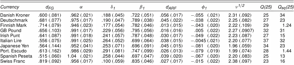
Table 1. The ARFI-HYGARCH Model of Exchange Rates

Currency d_FG ® ±₁ ¯₁ d_ARF Á₁ º1=2 _{Q(25) Q}

sq(25)

Danish Kroner :600.:081/ :962.:021/ :188.:045/ :722.:051/ :056.:017/ ¡:055 .:021/ 2:31.:092/ 25 34 Deutschmark :681.:077/ :975.:017/ :190.:047/ :789.:038/ :045.:022/ _¡:038 .:022/ 2:25.:082/ 27 23 Finnish Mark :714.:079/ :946.:023/ :177.:054/ :782.:046/ :013.:015/ ¡:043 .:020/ 2:22.:109/ 29 1:24 GB Pound :656.:103/ :991.:017/ :229.:056/ :795.:056/ :016.:016/ :005 .:022/ 2:27.:0907/ 32 31 Irish Punt :641.:087/ :991.:018/ :241.:057/ :787.:048/ :030.:017/ ¡:049 .:022/ 2:23.:087/ 27 15 Italian Lire :556.:075/ :991.:025/ :264.:052/ :699.:064/ :038.:015/ ¡:0045.:021/ 2:20.:077/ 37 32 Japanese Yen :564.:144/ :952.:041/ :253.:071/ :696.:091/ :045.:015/ ¡:081 .:020/ 1:96.:059/ 34 23 Port. Escudo :613.:162/ :986.:029/ :291.:081/ :747.:099/ :026.:013/ ¡:079 .:019/ 1:99.:074/ 28 1:44 Spanish Peseta :515.:060/ 1:04 .:021/ :258.:044/ :697.:047/ :039.:020/ ¡:067 .:020/ 2:20.:083/ 25 13 Swiss Franc :819.:092/ :956.:017/ :100.:059/ :835.:046/ :027.:017/ ¡:015 .:022/ 2:38.:097/ 23 16

NOTE: Robust standard errors are given in parentheses.

the Gaussian log-likelihood, but large innovations, such that u2_t=.º _¡2/htÀ1, make a much smaller contribution to the

ag-gregate than in the Gaussian case, depending on the size ofº. The last two columns of Table 1 show the Box–Pierce (1979) Q.r/statistic for r_D 25 lags, as well as theQsq, theQ

sta-tistic computed from the squared residuals. This test was pro-posed by McLeod and Li (1983) and studied by Li and Mak (1994) for application to testing neglected heteroscedasticity in ARCH residuals. Li and Mak showed that using the nominal chi-squared distribution with rdegrees of freedom would give an excessively conservative test, similar to the Box–Pierce re-sult for ARMA residuals. The asymptotic distributions of these statistics for the cases of hyperbolic lags in mean and variance have not yet been studied, so both must be treated with cau-tion, as diagnostic tests. What can be stated is that examina-tion of the residual correlograms in each case tends to show the largest (absolute) values at rather high lags (10 or 15 is typical). The neglected autocorrelation, in levels or squares, thus can-not be accounted for by simply adding terms to the ARMA or GARCH components, a conclusion reinforced by conventional signiŽcance tests.

Caution must also be observed in interpreting conventional conŽdence intervals, because although the samples are large, the asymptotic properties of the estimates are not yet well established. Lumsdaine (1996) and Lee and Hansen (1994) considered the IGARCH(1;1) case and showed that covari-ance stationarity of the processes is not a necessary condition for consistency and asymptotic normality of the usual quasi-maximum likelihood. However, note that the conjecture of Baillie et al. (1996, p. 9), to the effect that the properties of the FIGARCH model are subsumed under those of the IGARCH model, is in doubt in view of the analysis of this article.

Even with these caveats in mind, these results show a remark-able degree of uniformity. The point estimates of each parame-ter seem to differ by hardly more than the sampling error to be expected from identical data-generation processes. Because these are rates of exchange determined in closely related mar-kets, this perhaps is not unexpected. Some of these currencies were, of course, in the Exchange Rate Mechanism for some part of the sample period, and to the extent that they were tied together, they may be expected to move similarly against the dollar. However, the exceptional cases (Yen, Swiss franc) do not appear to diverge from the general pattern. It therefore can be conjectured that the similarity of these structures goes deeper than the fact of some correspondence in their movement in levels.

Looking now at the estimates themselves, note that although thedARFestimates are small, they are generally signiŽcant. On

the other hand, the hyperbolic memory in variance, measured bydFG, is generally pronounced. In most cases the amplitude

parameter ® is not signiŽcantly different from 1, while gen-erally a little below it. The FIGARCH model explains these data pretty well. Also, note that the estimate of d for the Deutschmark is similar to the FIGARCH estimations reported by Baillie et al. (1996) and also Beltratti and Morana (1999). A noteworthy feature is that the Studenttdegrees-of-freedom parameter,º, is generally close to its lower bound, correspond-ing toº1=2>1:414.

6.2 The Asian Crisis

The second application considered is to the dollar exchange rates for three Asian currencies, for periods covering the Asian crisis of 1997–1998. The series in question, in logarithms, are shown in panels (a) of Figures 1–3. At Žrst sight, it might ap-pear that these data represent two quite distinct regimes. Before the crisis, the Won and the Rupiah, at least, appear to be follow-ing a creepfollow-ing peg to the dollar; after the crisis, they are oatfollow-ing and subject to violent uctuations. The hypothesisthat the same time series model might account for both periods is evidently a strong one. However, it is not wholly unreasonable. These models may be seen as representing mechanisms by which ex-change markets Žlter new information, in the process of form-ing a price. The new information takes the form, by hypothesis (or by deŽnition, even), of an independent random sequence. The distribution of this sequence, and the time series model, are distinct contributing factors in the formation of the series. It may be that when unusual events occur the model changes, but a simpler hypothesis is that it does not.

Tables 2–4 show estimated models for the three currencies. The models were selected by individual speciŽcation searches on the complete samples, and parameters not shown in the ta-bles were restricted to 0. Lagrange multiplier (LM) statistics for the exclusion of some additional dynamic parameters are shown, to justify these choices. The intercepts in the mean processes were never signiŽcantly different from 0 when Žtted,

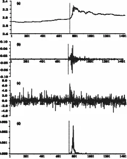
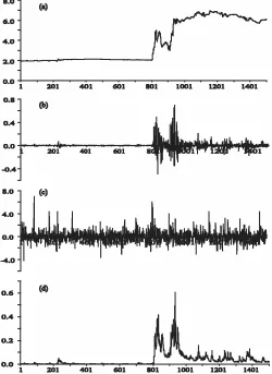
Figure 1. Korean Won. (a) Korean Won/US Dollar exchange rate (logarithms), observed time series; (b) unadjusted residuals (uO_t), model in Table 2, Column 1; (c) adjusted residuals (uO_t=¾O_t), model in Table 2, Column 1; and (d) conditional variances (¾O2

t ), model in Table 2,

Col-umn 1.

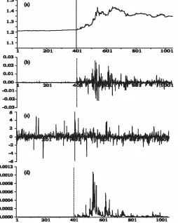
Figure 2. Indonesian Rupiah. (a) Indonesian Rupiah/US Dollar ex-change rate (logarithms), observed time series; (b) unadjusted resid-uals (uO_t), model in Table 3, Column 1; (c) adjusted residuals (uO_t=¾O_t), model in Table 3, Column 1; and (d) conditional variances (¾O_t2), model in Table 3, Column 1.

and are constrained to 0 in these estimates. Note that the fourth root of!has been estimated. Because!is close to 0 in these models, this transformation is found to improve numerical sta-bility, probably by giving better numerical approximations to derivatives.

Along with the full sample, the same models were also Žtted to “pre-crisis” and “post-crisis” subsamples. The breakpoints were in each case chosen by eye, at the point just preceding

Figure 3. Taiwan Dollar. (a) Taiwan Dollar/US Dollar exchange rate (logarithms), observed time series; (b) unadjusted residuals (uOt), model

in Table 4, Column 1; (c) adjusted residuals (uO_t=¾O_t), model in Table 4, Column 1; and (d) conditional variances (¾O_t2), model in Table 4, Col-umn 1.

the Žrst large fall of the currency. Using the methodology of Lavielle and Moulines (2000), Andreou and Ghysels (2002) de-tected multiple breaks in the volatility dynamics of stock mar-ket indices during the Asian crisis. However, in this instance there is inevitably a moment in the crisis at which the monetary authorities allow the currencies to oat freely, leading to precip-itate devaluations. It is these events that are taken to mark the regime switch dates. These are marked by the vertical lines in the Žgures, which show in panels (b), (c), and (d) respectively,

Table 2. Korean Won

12/13/94–6/15/00 12/13/94–10/16/97 10/17/97–6/15/00 (1,424 observations) (730 observations) (694 observations)

d_FG :669 .:046/ :667 .:121/ :686.:066/ ® 1:252 .:149/ 1:265 .:275/ 1:226.:177/ ¯₁ :339 .:092/ :318 .:143/ :363.:140/ !1=4 _{:0184.:0018/ :0186.:0026/ :021.:0091/} d_ARF :073 .:031/ :072 .:038/ :076.:059/ Á₁ :116 .:039/ :110 .:051/ :122.:068/ Á₂ ¡:097 .:028/ ¡:044 .:038/ ¡:152.:044/ º1=2 1:73 .:080/ 1:71 .:113/ 1:74 .:116/

Kurtosis 8.65 7.16 7.93

Q.25/ 44 21 34

Qsq.25/ 39 17 47

LM(±₁) .204 — —

Log likelihood 7,421.85 4,314.09 3,109.97

LR statistic (8 df)D4.42

NOTE: Robust standard errors are given in parentheses.

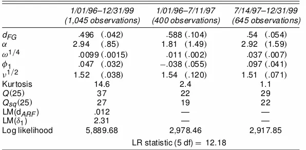
Table 3. Indonesian Rupiah

1/01/96–12/31/99 1/01/96–7/11/97 7/14/97–12/31/99 (1,045 observations) (400 observations) (645 observations)

d_FG :496 .:042/ :588.:104/ :54 .:054/ ® 2:94 .:85/ 1:81 .1:49/ 2:92 .1:59/ !1=4 :0099.:0015/ :011.:002/ :037.:007/ Á₁ :047 .:032/ ¡:038.:055/ :097.:041/ º1=2 1:52 .:038/ 1:54 .:120/ 1:51 .:071/

Kurtosis 14.6 2.4 1.1

Q.25/ 37 22 29

Qsq.25/ 27 19 22

LM(d_ARF) .012 — —

LM(±₁) 2.31 — —

Log likelihood 5,889.68 2,978.46 2,917.85

LR statistic (5 df)D 12.18

NOTE: Robust standard errors are given in parentheses.

the estimated series u_Ot, uOt=¾Ot, and ¾Ot2 from the HYGARCH

model in each case.

An examination of these results leads to three conclusions. First, the three structures estimated are not wholly dissimilar, but each has distinctive features. In particular, the Won exhibits quite a complex structure of autocorrelation, although this may be due to the fact that the higher leptokurtosis of the other two shock series has the effect of masking any autocorrelation that may be present. Second, however, they more closely resemble each other than the currencies analyzed in Table 1. The most noteworthy feature is, of course, the large values of the® para-meter in each case, especially for the Rupiah and Taiwan dollar. Third, and perhaps most remarkable, is the stability of these models across the pre-crisis and post-crisis regimes. In all three cases the large®value is common to both periods, and the other parameters are also generally close. The last line of each table shows the likelihood ratio statistic for the test of model stabil-ity across the sample. Note that this cannot be interpreted as an asymptotic chi-squared test, because the breakpoints have been chosen with reference to the data—that is, the most extreme contrast has been drawn in each case. Therefore, the correct null distribution of this statistic is the distribution of the maximum log-likelihood ratio over all breakpoints. These critical values must exceed the nominal chi-squared values. The statistic for the Won is actually within the nominal acceptance region for the 5% test, and that for the Rupiah is only slightly outside it. Overall, these results provide little evidence for changes in the

model following the crisis, and the residual plots in panels (c) of Figures 1–3 (from the model Žtted to the full sample) pro-vide another view of this epro-vidence. In two out of three cases, at least, it would appear impossible to detect the breakpoint with conŽdence “by eye.”

One further piece of evidence on the performance of these models is presented in Figure 4. This is a simulation using the model of the Korean Won, driven by shocks randomly re-sampled from the residuals of the same model, as shown in Figure 4(c). The data shown were generated after letting the process run for 2,000 presample periods, to remove dependence on initial conditions. A “crisis” was introduced by inserting into the (otherwise randomly drawn) sequence a succession of Žve positive shocks, beginning at period 801. The values arbitrar-ily chosen were 4.2, 6.0, 3.3, 2, and 5.1, expressed in standard deviations, because that of the shock distribution is 1 by con-struction. Such a realization would be a fairly rare event under random resampling, although major exchange crises are simi-larly rare, so this is not inappropriate.

There is, of course, no suggestion that the model (essen-tially, a heteroscedastic random walk) always generates runs of this appearance. Several repetitions of the experiment were required to produce the case illustrated, selected for its resem-blance to the observed data. The point to be made here is merely that the observed data, taken as a whole, arecompatiblewith this type of data-generation process. SpeciŽcally, the pre-crisis

Table 4. Taiwan Dollar

01/03/94–6/15/00 01/03/94–10/15/97 10/16/97–6/15/00 (1,683 observations) (988 observations) (695 observations)

d_FG :860.:079/ 1:001.:010/ :667 .:073/ ® 2:96 .:466/ 2:956.:466/ 2:946 .:877/ ±₁ :242.:138/ :009.:187/ :568 .:221/ ¯₁ :635.:043/ :606.:042/ :726 .:136/ !1=4 _{:021.:006/ :022.:006/ :000037.:004/}

Á₁ ¡:075.:024/ ¡:131.:031/ ¡:007 .:037/ º1=2 1:47 .:010/ 1:46 .:010/ 1:46 .:019/

Kurtosis 336 21 184

Q.25/ 9.40 49 5.27

Qsq.25/ .21 23 .11

LM(d_ARF) .037 — —

Log likelihood 8,631.47 5,263.64 3,38.61

LR statistic (7 df)D 25.56

NOTE: Robust standard errors are given in parentheses.

Figure 4. Korean Won Simulation. (a) Stochastically simulated se-ries, using model in Table 2, Column 1; (b) HYGARCH shocks of simu-lated series; (c) shocks randomly resampled from series in Figure 1(c), with inserted “crisis” at period 801; and (d) conditional variances of sim-ulated series.

“pegged-rate” segments of the series in Figures 1(a)–3(a), al-though possibly appearing “stationary,” are actually well ex-plained by a I(1_Cd) process, provided that the innovations are small enough. To switch to the post-crisis behavior, all that is required are some unusually large shocks and a conditional variance process with hyperbolic memory and large amplitude. As can be seen, the resulting pattern of high volatility can per-sist without further external stimulus, for scores and even hun-dreds of periods.

This analysis points to the possibility that the behavior of currency markets as Žlters of new information could be sim-pler in structure than many observers seem to believe. The natural rivals for the type of model presented here feature ex-ogenous variables, either measured variables or dummies in-dicating the new environment, or, alternatively, are Markov-switching (SWARCH) models in which the deus ex machina takes the form of an autonomous stochastic process to pro-vide the switching mechanism (see, e.g., Hamilton and Susmel 1994). What we aim to show is that although any of these may be the true explanations,there is noneedto introduce them. The crisis behavior can be well described by a very simple endoge-nous mechanism, driven solely by the information contained in the shock process itself.

7. CONCLUSION

In this article, conditions have been derived for the exis-tence of moments and near-epoch dependence of the general class of ARCH(₁) processes. This class includes the GARCH, IGARCH, and FIGARCH models, among other alternatives. It has been argued that the properties of these processes should be represented as varying in the two dimensions of amplitude and memory, relating to the magnitude of the sum of the lag coefŽ-cients and their rate of convergence. The proposed HYGARCH model generalizes the FIGARCH model to permit both the exis-tence of second moments on the one hand, and greater extremes of amplitude on the other. Application of the model to exchange rates is illustrated by two contrasting sets of examples.

An important implication of the results is the danger of press-ing too far the analogy between integrated (i.e., fractional) mod-els in levmod-els, and modmod-els whose conditional variances have an apparently similar dynamic structure. The relationship between the degree of persistence and the wide-sense stationarity of the process obeys very different rules in the two cases. The IGARCH is a short-memory process having no variance, the FIGARCH(d) model has shortest memory withd closest to 1, and in general ARCH(₁) processes can be persistent and yet wide-sense stationary.

A further implication is the inability of the ARCH(₁) class to represent the degree of persistence commonly called “long memory.” An interesting commentary on this question is pro-vided by Andersen and Bollerslev (1997), who considered a semiparametric model in which the spectrum of absolute re-turns is treated as unbounded at the origin, diverging like_j!_j¡2d

for a parameter d>0, as!_!0. Their d was estimated by the method of Geweke and Porter-Hudak (1983) from high-frequency data under varying degrees of time aggregation. It is important to stress that this d parameter is different from thed parameter deŽned by (9) or (34). A spectrum diverging at the origin implies nonsummable autocorrelations, which are not permitted in the ARCH(₁) framework. If true long mem-ory in variance is to be represented parametrically, it will have to be in the context of a different class of models.

The exponential ARCH(₁) class, in which loght is

mod-eled by a distributed lag of some appropriate indicator of re-alized volatility, could be a plausible candidate for this role. Andersen and Bollerslev (1997) derived an exponential model, but also argued that persistence characteristics should be pre-served under monotone-increasing transformations, so that the spectrum of absolute returns should capture the same long-memory characteristics. The EGARCH model of Nelson (1991) may be taken as a case in point. Here loghtis represented as an

inŽnite moving average of a functiong.et/, whereet is the iid

driving process. If (34) were allowed to represent (in a purely formal way) the lag structure in this model, then the interpre-tation of the coefŽcients® anddwould, of course, be entirely different. In particular,® would be irrelevant to the existence of moments, andd<0 (such that the lag coefŽcients are not absolutely summable) would not necessarily be incompatible with stationarity. One might even speculate that the parame-ter estimated by Andersen and Bollerslev (1997) corresponds to_¡din this setup. Investigating these issues goes well beyond the scope of this article, but represents an interesting avenue for further research.

ACKNOWLEDGMENTS

This research was supported by the ESRC under award L138251025.The author is most grateful to an anonymous ref-eree for suggestions for simplifying the proofs for Section 3, and also to Soyeon Lee for providing useful comments and also the Asian crisis datasets used in Section 6.2.

APPENDIX: PROOFS OF THEOREMS A.1 Proof of Theorem 1

Because¾_t2_¸!andE_tt_¡C_mm¾_t2_¸!, the inequality

kut¡Ett_¡Cmmutkp·!¡1=2k¾t2¡Ett_¡Cmm¾t2kp

follows by a minor extension of lemma 4.1 of Davidson (2002), replacing 2 withp_¸1. Therefore, in view of stationarity, it suf-Žces to prove the inequalities

k¾_t2_¡Et_t¡C_mm¾_t2_kp·Cpm¡± (A.1)

forCp>0, forpD1 andpD2. Repeated substitution leads to,

for givenm, the decomposition

¾_t2_D!_C

To prove part (a), Žrst note that

E­­e2_t¡j using the Jensen inequality and law of iterated expectations in the second case. Similarly,

whereM2is deŽned after (15). Next, deŽne

TpD

To prove part (b), note similarly that

®

A.2 Proof of Theorem 2

The proof of Theorem 1 is modiŽed as follows. For part (a), note that because½ >1 andS<1, there exists" >0 such that

· QCp½_Q¡mSQp

A.3 Proof of Theorem 3

Let

dence of these terms ontis implicit but not indicated for ease of notation. By subadditivity,

P._j¾_t2_¡hm_{t j}> ±/_·P.!_jU1C¢ ¢ ¢CUmj> ±=2/CP.Vm> ±=2/;

and the approach is to bound each term separately. First, note thatE_jUpj DTp, as deŽned in (A.4). Under the assumptions,

where" >0 is to be chosen. [Note that although (A.7) is similar to the expression in (A.3), here the sign on"is reversed, and in this case the sum may exceed 1.] By subadditivity,note that

P.Vm> ±=2/

Rewrite the probabilities in (A.8) in the form

P¡e2_t¡j

form_D1;2; : : : :Because theet are iid random variables, the

CLT implies that for large m, the distribution of the sum is approximately Gaussian with mean _¡m³ and variancem¿2, where¿2_Dvar.loge2_t/. Note that by the Jensen inequality,

³ _{D ¡}E.loge2_j/ >_¡logE.e2_j/_D0:

Hence, for large enoughm,

N

Here the second equality is obtained, assuming that

logB.j1; : : : ;jmC1/Cm³ >0

(to be established below) from the asymptotic expansion of the Gaussian probability function, (see 26.2.12 of Abramowitz and Stegun 1965). Note that the error in the expansion is condition-ally ofO.m¡2/.

Because_flog¾_t2_gis a stationary sequence by assumption, and henceOp.1/,

Asmincreases, the conditional probability expression in (A.9) (suitably renormalized so that it does not vanish) is con-verging in probability to a nonstochastic limit, which neces-sarily matches that of the large-m unconditional probability. Henceforth, this formula is modiŽed by neglecting the terms ofOp.1=m/. First, note that

fore always positive if³ >logSQ, which henceforth is assumed. Next, note that

Combining (A.8)–(A.11) yields, for large enoughm,

P.Vm> ±=2/

For the right side expression to vanish asm_{! 1}requires that the sum of terms in parentheses in the exponent be positive. Using³ >logSQ, the sufŽcient condition,

3 log2SQ>2¿2logSL; (A.12)

By taking"large enough, this can be made arbitrarily close to

3¡.1_C"/2.logC_¡log½ /¢2>2."³logC_¡"³log½/ >2".logC_¡log½/2;

which holds for any choice ofCand½. It follows that³ >logSQ is sufŽcient, which proves part (b) of the theorem. In turn, C< ½ ensures that logSQ _·0 for large enough" >0, which proves part (a).

[Received June 2001. Revised April 2003.]

REFERENCES

Abramowitz, M., and Stegun, I. A. (1965),Handbook of Mathematical

Func-tions, New York: Dover Publications.

Andersen, T. G., and Bollerslev, T. (1997), “Heterogeneous Information Ar-rivals and Return Volatility Dynamics: Uncovering the Long Run in High

Volatility Returns,”Journal of Finance, 3, 975–1005.

Andreou, E., and Ghysels, E. (2002), “Detecting Multiple Breaks in

Finan-cial Market Volatility Dynamics,” Journal of Applied Econometrics, 17,

579–600.

Baillie, R. T., Bollerslev, T., and Mikkelsen, H. O. (1996), “Fractionally

Inte-grated Generalized Autoregressive Conditional Heteroscedasticity,”Journal

of Econometrics, 74, 3–30.

Baillie, R. T., Cecen, A. A., and Han, Y.-W. (2000), “High-Frequency Deutsche mark–U.S. Dollar Returns: FIGARCH Representations and

Non-Linearities,”Multinational Finance Journal, 4, 247–267.

Baillie, R. T., and Osterberg, W. P. (2000), “Deviations From Daily Uncovered

Interest Rate Parity and the Role of Intervention,”Journal of International

Financial Markets Institutions and Money, 10, 363–379.

Beltratti, A., and Morana, C. (1999), “Computing Value at Risk With

High-Frequency Data,”Journal of Empirical Finance, 6, 431–455.

Bollerslev, T. (1986), “Generalized Autoregressive Conditional

Heteroscedas-ticity,”Journal of Econometrics, 31, 307–327.

Box, G. E. P., and Pierce, D. A. (1970), “The Distribution of Residual Autocor-relations in Autoregressive-Integrated Moving Average Time Series

Mod-els,”Journal of the American Statistical Association, 65, 1509–1526.

Brunetti, C., and Gilbert, C. L. (2000), “Bivariate FIGARCH and Fractional

Cointegration,”Journal of Empirical Finance, 7, 509–530.

Davidson, J. (1994),Stochastic Limit Theory—An Introduction for Econome-tricians, Oxford, U.K.: Oxford University Press.

(2002), “Establishing Conditions for the Functional Central Limit

The-orem in Nonlinear and Semiparametric Time Series Processes,”Journal of

Econometrics, 106, 243–269.

(2003), “Time Series Modelling, Version 3.1,” available at

www.cf.ac.uk/carbs/econ/davidsonje/software.html.

De Jong, R. M. (1997), “Central Limit Theorems for Dependent Heterogeneous

Processes,”Econometric Theory, 13, 353–367.

Ding, Z., and Granger, C. W. J. (1996), “Modelling Volatility Persistence

of Speculative Returns: A New Approach,”Journal of Econometrics, 73,

185–215.

Doornik, J. A. (1999), Object-Oriented Matrix Programming Using Ox

(3rd ed.), London: Timberlake Consultants Press.

Engle, R. F. (1982), “Autoregressive Conditional Heteroscedasticity With

Es-timates of the Variance of United Kingdom Ination,”Econometrica, 50,

987–1007.

Engle, R. F., and Bollerslev, T. (1986), “Modelling the Persistence of

Condi-tional Variances,”Econometric Reviews, 5, 1–50.

Geweke, J., and Porter-Hudak, S. (1983), “The Estimation and Application

of Long-Memory Time Series Models,”Journal of Time Series Analysis, 4,

221–238.

Giraitis, L., Kokoszka, P., and Leipus, R. (2000), “Stationary ARCH Models:

Dependence Structure and Central Limit Theorem,”Econometric Theory, 16,

3–22.

Granger, C. W. J. (2002), “Long Memory, Volatility, Risk and Distribution,” working paper, University of California San Diego, Dept. of Economics.

Granger, C. W. J., and Teräsvirta, T. (1993),Modelling Nonlinear Economic

Relationships, Oxford, U.K.: Oxford University Press.

Hamilton, J. D., and Susmel, R. (1994), “Autoregressive Conditional

Het-eroscedasticity and Changes in Regime,” Journal of Econometrics, 64,

307–333.

He, C., and Teräsvirta, T. (1999), “Fourth-Moment Structure of the

GARCH(p;q) Process,”Econometric Theory, 15, 824–846.

Karonasos, M. (1999), “The Second Moment and the Autocovariance Function

of the Squared Errors of the GARCH Model,”Journal of Econometrics, 90,

63–76.

KazakeviÏcius, V., and Leipus, R. (2002), “On Stationarity in the ARCH(1)

Model,”Econometric Theory, 18, 1–16.

Lavielle, M., and Moulines, E. (2000), “Least Squares Estimation of an

Un-known Number of Shifts in Time Series,”Journal of Time Series Analysis,

20, 33–60.

Lee, S.-W., and Hansen, B. E. (1994), “Asymptotic Theory for the

GARCH(1;1) Quasi-Maximum Likelihood Estimator,”Econometric Theory,

10, 29–52.

Li, W. K., and Mak, T. K. (1994), “On the Squared Residual Autocorrelation

in Nonlinear Time Series With Conditional Heteroscedasticity,”Journal of

Time Series Analysis, 15, 627–636.

Lumsdaine, R. L. (1996), “Consistency and Asymptotic Normality of the

Quasi-Maximum Likelihood Estimator in IGARCH(1;1) and Covariance

Stationary GARCH(1;1) Models,”Econometrica, 64, 575–596.

McLeod, A. I., and Li, W. K. (1983), “Diagnostic Checking ARMA Time Series

Models Using Squared-Residual Autocorrelations,”Journal of Time Series

Analysis, 4, 269–273.

Nelson, D. B. (1990), “Stationarity and Persistence in the “GARCH(1;1)

Model,”Econometric Theory, 6, 318–334.

(1991), “Conditional Heteroscedasticity in Asset Returns: A New

Ap-proach,”Econometrica, 59, 347–370.

Pötscher, B. M., and Prucha, I. R. (1991), “Basic Structure of the Asymptotic Theory in Dynamic Nonlinear Econometric Models, Part I: Consistency and

Approximation Concepts,”Econometric Reviews, 10, 125–216.