Full Terms & Conditions of access and use can be found at
http://www.tandfonline.com/action/journalInformation?journalCode=ubes20
Download by: [Universitas Maritim Raja Ali Haji] Date: 12 January 2016, At: 17:43
Journal of Business & Economic Statistics
ISSN: 0735-0015 (Print) 1537-2707 (Online) Journal homepage: http://www.tandfonline.com/loi/ubes20
Monotonic Regression Based on Bayesian
P–Splines
Andreas Brezger & Winfried J Steiner
To cite this article: Andreas Brezger & Winfried J Steiner (2008) Monotonic Regression Based on Bayesian P–Splines, Journal of Business & Economic Statistics, 26:1, 90-104, DOI: 10.1198/073500107000000223
To link to this article: http://dx.doi.org/10.1198/073500107000000223
Published online: 01 Jan 2012.
Submit your article to this journal
Article views: 153
View related articles
Monotonic Regression Based on Bayesian
P–Splines: An Application to Estimating
Price Response Functions From
Store-Level Scanner Data
Andreas BREZGER
Department of Statistics, University of Munich, Munich, Germany
Winfried J. STEINER
Department of Marketing, Institute of Management and Economics, Technical University of Clausthal, Clausthal-Zellerfeld, Germany (winfried.steiner@tu-clausthal.de)
In many practical situations, it is desirable to restrict the flexibility of nonparametric estimation to accom-modate a presumed monotonic relationship between a covariate and the response variable. We follow a Bayesian approach using penalized B-splines and incorporate the assumption of monotonicity in a natural way by an appropriate specification of the respective prior distributions. We illustrate the methodology in an empirical application modeling demand for brands of orange juice and show that imposing monotonic-ity constraints for own- and cross-item price effects improves the predictive validmonotonic-ity of the estimated sales response functions considerably.
KEY WORDS: Asymmetric quality tier competition; Generalized additive model; Markov chain Monte Carlo; Own- and cross-item price effects; Sales promotion.
1. INTRODUCTION
Generalized additive models (GAMs) are a powerful tool for modeling possibly nonlinear effects of multiple covariates. For continuous covariates, the variety of different approaches for nonlinear modeling comprises, for example, smoothing splines (e.g., Hastie and Tibshirani 1990), regression splines (e.g., Friedman and Silverman 1989; Friedman 1991; Stone, Hansen, Kooperberg, and Truong 1997), local methods (e.g., Fan and Gijbels 1996) as well as P-splines (Eilers and Marx 1996; Marx and Eilers 1998). Bayesian nonparametric approaches make use of adaptive knot selection (e.g., Smith and Kohn 1996; Denison, Mallick, and Smith 1998; Biller 2000; Di Matteo, Genovese, and Kass 2001; Biller and Fahrmeir 2001; Hansen and Kooper-berg 2002) or smoothness priors (Hastie and Tibshirani 2000; Fahrmeir and Lang 2001a,b). Lang and Brezger (2004) have adopted the frequentist P-splines of Eilers and Marx (1996) for a Bayesian framework for additive models and Brezger and Lang (2005) have extended their work to GAMs.
Whereas strictly parametric modeling is too restrictive in many cases, the flexibility of non- and semiparametric ap-proaches may lead to implausible results on the other hand. Clearly, the problem of overfitting can be addressed by penal-ization of too rough functions or by adaptive knot selection. Much less discussed in the literature on nonparametric estima-tion is, however, the important case when theory and/or em-pirical evidence strongly suggest a monotonic relationship be-tween a covariate and a response variable. For example, con-sumers usually will buy less of a brand as its price increases, and therefore one expects a brand’s unit sales or market share to decrease monotonically in price. The downward slope of own-price response functions is in accordance with economic the-ory (e.g., Rao 1993), and there is strong empirical support that own-price elasticities are negative and elastic (e.g., Tellis 1988;
Hanssens, Parsons, and Schultz 2001). Similarly, we generally expect cross-price effects on competitive items (i.e., brand sub-stitutes) to be positive or at least nonnegative, implying that a price cut by one brand may decrease but by no means will in-crease the unit sales of competitive brands (Sethuraman, Srini-vasan, and Kim 1999). Examples for presumed monotonic re-lationships can also be found in disciplines other than business and economics, as it is the case for many dose-response rela-tionships in medicine. For instance, the concentration of dust and the duration of exposure to it at work is assumed to af-fect the occurrence of certain lung diseases in a monotonic way (Ulm and Salanti 2003). Monotonic effects are also referred to as isotonic if the respective function is nondecreasing, and an-titonic if a function is nonincreasing.
The topic of monotonic regression has already been ad-dressed by Ramsay (1988, 1998), Ulm and Salanti (2003), and Salanti and Ulm (2003) in a frequentist setting. Allenby, Arora, and Ginter (1995) have incorporated prior ordinal in-formation about regression parameters of dummy coded co-variates in a Bayesian setting. Specifically, they have proposed a Bayesian model for conjoint analysis with order restrictions (monotonicity constraints) for part-worth utilities. Dunson and Neelon (2003) and Holmes and Heard (2003) have presented further Bayesian approaches to monotonic regression. The for-mer, however, have considered only GLMs and modeling has been based on piecewise constant functions, while the latter have dealt with only a small number of level sets obtained from a categorization of continuous covariates.
In this article we propose to use Bayesian P-splines of an arbitrary degree and enforce monotonicity with an additional
© 2008 American Statistical Association Journal of Business & Economic Statistics January 2008, Vol. 26, No. 1 DOI 10.1198/073500107000000223 90
restriction. This restriction may be imposed for either one or an arbitrary number of the additive terms in the model, whereas other terms may be modeled unrestricted. Markov chain Monte Carlo (MCMC) inference involves sampling from multivariate truncated normal distributions. This is accomplished by an “in-ternal” Gibbs sampler in each iteration; that is, we employ a short Gibbs sampler to draw from the proposal density. In the non-Gaussian case, we draw from an iteratively weighted least squares (IWLS) proposal density in a Metropolis–Hastings step. Our methodology is implemented with the public domain software packageBayesX(Brezger, Kneib, and Lang 2005). It is possible to combine monotonic regression with all types of response distributions supported byBayesX. These are the most common one-dimensional distributions such as Gaussian, Bino-mial, Poisson, Gamma, and Negative BinoBino-mial, and multino-mial logit and cumulative probit models for multivariate re-sponses.BayesXalso supports the use of random effects to ac-count for unobserved heterogeneity, Gaussian Markov random field (GMRF) priors for spatial covariates, and varying coef-ficient terms and surface smoothing for interactions of covari-ates.
The remainder of the article is organized as follows: Sec-tion 2 briefly reviews GAMs and (Bayesian) P-splines, whereas Section 3 provides details on the MCMC techniques employed. In Section 4 we apply the proposed methodology to weekly store-level scanner data to relate unit sales of a particular brand of orange juice in a major supermarket chain to own and com-peting brands’ promotional instruments. Using a lognormal model and a Gamma model, we illustrate for both Gaussian and non-Gaussian responses that imposing monotonicity con-straints on the nonparametric terms for own-item and cross-item price effects improves the predictive validity of the esti-mated sales response functions considerably. In Section 5 we present some refinements of our methodology, including a re-laxation of our MCMC procedure to impose monotonicity as well as a sensitivity analysis on the number and position of knots used for the P-splines. We further apply our methodol-ogy to a second brand (the supermarket’s private label brand) to validate our findings obtained in Section 4. We conclude with a summary of the most important contents and key findings in Section 6.
2. MODEL ASSUMPTIONS
2.1 Generalized Additive Models and P–Splines
Suppose we are given N observations (yn, xn, vn), n=
1, . . . , N, whereynis a response variable,xn=(xn1, . . . , xnp)′
is a vector of continuous covariates, andvn=(vn1, . . . , vnq)′is
a vector of additional covariates. GAMs assume that, givenxn
andvn, the responseynfollows an exponential family
distribu-tion (Hastie and Tibshirani 1990; Fahrmeir and Tutz 2001)
p(yn|xn, vn)=c(yn, φ)exp
ynθn−b(θn) φ
, (1)
where b(·), c(·),θn, and φ define the respective distribution
[e.g., ifb(θn)=θn2/2, c(yn, φ)=exp(y2n/(2φ))/
√
2π φ,θn= μn, andφ=σ2, we obtain an N(μn, σ2)distribution]. GAMs
further assume that the mean μn=E(yn|xn, vn) is linked to
a semiparametric additive predictorηnvia a known link
func-tiong:
g(μn)=ηn, ηn=f1(xn1)+ · · · +fp(xnp)+vn′γ . (2) f1, . . . , fpare unknown smooth functions of the continuous
co-variates andvn′γ represents the parametric part of the predictor. For modeling the unknown functionsfj, j =1, . . . , p, we
follow Lang and Brezger (2004), who proposed a Bayesian ver-sion of the P-splines approach introduced in a frequentist set-ting by Eilers and Marx (1996). Accordingly, we assume that the unknown functions can be approximated by a polynomial spline of degreeland withk+1 equally spaced knots
xj,min=ζj0< ζj1<· · ·< ζj,k−1< ζj k=xj,max (3) over the domain of xj. The spline can be written in terms of
a linear combination of =k+l B-spline basis functions (De Boor 2001). Figure 1 gives an illustration of B-spline ba-sis functions of degree 3, which are also referred to as cubic splines. Explicit formulas for the functional form of B-spline basis functions are given in Appendix A. Note that except at the boundaries each basis function overlaps with 2·l neighbor-ing B-splines (i.e., with six neighborneighbor-ing B-splines in the case of cubic splines; see Fig. 1).
Denoting theψth basis function byBj ψ, we obtain
fj(xj)=
ψ=1
βj ψBj ψ(xj). (4)
Figure 1. B-spline basis functions of degree 3 covering the interval[A, B].
To keep notation simple, we assume an equal number of basis functions for all functionsfj. By defining theN× design
matricesXj, where the element in rownand columnψis given
by Xj(n, ψ )=Bj ψ(xnj), we can rewrite the predictor (2) in
matrix notation as
η=X1β1+ · · · +Xpβp+V γ . (5)
Here βj =(βj1, . . . , βj )′, j =1, . . . , p, corresponds to the
vector of unknown regression coefficients. The matrixV is the usual design matrix for parametric effects. To overcome the dif-ficulties in determining the position and the number of the knots involved with regression splines, Eilers and Marx (1996) sug-gested a relatively large number of knots (usually between 20 and 40) to ensure sufficient flexibility, and to introduce a rough-ness penalty of first- or second-order differences on adjacent regression coefficients to avoid overfitting. These penalized B-splines have also become known as P-B-splines. In our Bayesian approach, we replace first- or second-order differences used in this frequentist approach with their stochastic analogues, that is, first- or second-order random walks defined by
βj ψ =βj,ψ−1+uj ψ or
(6)
βj ψ =2βj,ψ−1−βj,ψ−2+uj ψ
with Gaussian errorsuj ψ∼N(0, τj2)and diffuse priorsβj1∝
const, or βj1 andβj2∝const, for initial values, respectively. The amount of smoothness is controlled by the variance para-meter τj2, which corresponds to the inverse of the smoothing parameter in the frequentist approach. The amount of smooth-ness can be estimated simultaneously with the regression co-efficients by defining an additional hyperprior for the variance parametersτj2.
We assign the conjugate prior forτj2(and for the scale pa-rameterσ2in the Gaussian case) which is an inverse Gamma distribution
τj2∼IG(aj, bj) (7)
with hyperparametersaj andbj. A common choice foraj and bj leading to almost diffuse priors is aj =bj, for example, aj=bj=.001, which is also our default choice. Alternatively,
we may set aj =1 andbj small, for example,bj =.005 or bj=.0005. We estimated all models discussed in this article
with alternative settings for the hyperparameters. The results proved to be almost insensitive regarding the specific choice of hyperparameters. All results presented in the remainder of the article are obtained by the default choice.
The random walks defined as priors for the individual basis functions according to (6) can be combined in a global smooth-ness prior. Taking into account that we use diffuse priors for the initialδparameters (i.e.,δ=1 orδ=2 corresponding to a first- or second-order random walk, respectively), we can write (6) equivalently asDδβj∼N(0, τj2I −δ), whereDδis a
differ-ence matrix of orderδ and dimension( −δ)× , andI −δ
is an identity matrix of dimension( −δ). Hence, by defining the penalty matrixKδ=Dδ′Dδ, we can formulate the prior for a P-spline term as a joint prior distribution forβj:
p(βj)∝exp
see Lang and Brezger (2004) for details. For example, forδ=1 we get
with zero elements outside the first off-diagonals.
2.2 Monotonicity Constraints
To obtain monotonicity, that is,fj′(x)≥0 orfj′(x)≤0, it is sufficient to guarantee that subsequent parameters are ordered, such that
βj1≤ · · · ≤βj or βj1≥ · · · ≥βj , (10)
respectively. A proof can be found in Appendix B. In our ap-proach, these constraints are imposed by introducing indicator functions to truncate the prior appropriately to obtain the de-sired support. This leads to
p(βj)=c1(βj)exp for nondecreasing functions (isotonic case) and
p(βj)=c1(βj)exp for nonincreasing functions (antitonic case), respectively, where
c1(βj)is a normalizing function depending onβj.
2.3 Extensions
Various extensions regarding the additive predictor (2) are possible. To account for unobserved heterogeneity between dif-ferent groups or clusters of units, we may add an unstructured group-specific random effect. Suppose we are given a grouping variable that can take values in{1, . . . , G}. Then, we can extend (2) to
ηn=f1(xn1)+ · · · +fp(xnp)+vn′γ+frandom(gn) (13)
and assume
frandom(g)=bg∼N(0, τb2), g=1, . . . , G, (14)
where frandom(gn)=frandom(g) if observation n belongs to groupg. Using the penalty matrixKb=I, we can write (14) in
If we would presume a spatial correlation between groups, we may additionally introduce a spatial correlated GMRF. Further possible extensions are varying coefficient terms and interac-tions of covariates (see Lang and Brezger 2004; Brezger and Lang 2005). In the remainder, we focus on models with ran-dom effects.
3. MCMC INFERENCE
Letα be the vector of all parameters to be estimated in the model. Bayesian inference is based on the posterior distribution
p(α|y)∝L(y, β1, . . . , βp, γ , bg, φ)
whereL(·)consists of the product of all individual likelihood contributions.φandp(φ)have to be omitted for response dis-tributions without a scale parameter. Because (16) is analyti-cally intractable in all but the most simple cases, we employ MCMC techniques to obtain estimates for the parameters of interest. More specifically, we implement a block move, that is, we subsequently draw from the full conditionals p(βj|·), j =1, . . . , p,p(γ|·), andp(bg|·)of the blocks of parameters βj, j =1, . . . , p, γ, and bg. For Gaussian responses, these
blocks can be updated by block-move Gibbs sampling steps. In binary probit and cumulative probit models, we can rely on the same sampling scheme as building block; see Chen and Dey (2000) or Brezger and Lang (2005) for details. In all other cases, we use Metropolis–Hastings steps with IWLS proposals. The variance parametersτ12, . . . , τp2,τb2(and the scale parameterσ2
in the Gaussian case) are updated by single-move Gibbs sam-pling steps.
For posterior inference, we discard the draws from an initial burn-in period and take only everyrth draw thereafter to mini-mize the autocorrelation of the samples. The formulas and algo-rithms in the following subsections are formulated with respect to isotonic constraints. The adjustments for antitonic constraints are straightforward.
3.1 Gaussian Response
For Gaussian response, the posterior distribution for βj is
given by
To sample from this -dimensional truncated Gaussian dis-tribution (17), we adopt the method of Robert (1995) and run an extra (short) single-move Gibbs sampler in each MCMC it-eration. The algorithm is as follows:
(a) Setβ(0)=βjc.
meanμ, varianceσ2and with left truncation pointμl and right
truncation point μr, respectively. The truncation points in the
algorithm above are the current states of the adjacent parame-ters. Therefore, we have only right truncation forβ1(t )and left truncation forβ(t ). The parametersμψandσψ2,ψ=1, . . . , ,
are the conditional means and variances of the (nontruncated) posterior (17):
rowψ and columnρ of the precision matrixPj in (17). Note
that the subscriptj is suppressed in the formulas above. (c) Takeβ(T )=(β1(T ), . . . , β(T ))′ as a random sample from (17).
Usually, convergence is reached after 10–20 cycles. To reach convergence with considerable certainty, we setT =100. Com-putation is very fast, as the meanmj and the precision matrix Pj have to be computed only once. Moreover,mj is obtained
by sparse matrix operations exploiting the band structure ofPj.
This involves a Cholesky decomposition and avoids expensive matrix inversions (cf. Rue 2001).
Regarding the parametric effects, we obtain a normal distri-bution with precision matrix and mean
Pγ =
1
σ2V
′V , m
γ =(V′V )−1V′(y−η+V γ ) (20)
as full conditional, if we use constant priors for the parameters
γ. Of course, a highly dispersed Gaussian distribution can be assigned as a conjugate prior as well when a priori information is sparse/lacking.
The full conditionals for the variance parameters τj2, j =
1, . . . , p,τb2, and the scale parameterσ2are all inverse Gamma
forσ2, whereǫis the usual vector of residuals.
3.2 Non-Gaussian Response
For non-Gaussian response, the posteriorp(βj|·)is
p(βj|·)∝c(yn, φ)exp
which has no longer standard form [e.g., if we consider a Gamma distribution with parametersμandν, as in our empir-ical application, this implies b(θn)= −log(−θn), c(yn, φ)= (φ−1)(φ−1)ynφ−1−1/ Ŵ(φ−1),θn= −1/μ, and φ=ν−1]. Thus,
we use a Metropolis–Hastings step with an IWLS proposal to update βj. An IWLS proposal is obtained by a quadratic
ap-proximation of the likelihood via Taylor expansion around the current state βjc of βj (cf. Brezger and Lang 2005 or, in the
mixed model context, Gamerman 1997). This leads to a trun-cated multivariate Gaussian proposal
expansion, which would simplify the calculation of the accep-tance probability; compare Brezger and Lang (2005). The main difference to the Gaussian sampling scheme is that this sample can only be accepted with probability
α(βjc, βjp)=min
as the new state ofβj. Note that the indicator functions involved
(in the prior and in the proposal) cancel out.
The full conditionals for the variance parameters τj2, j =
1, . . . , p, and τb2 are again inverse Gamma distributions and therefore updated via Gibbs sampling. Parametric effects are updated by Metropolis–Hastings steps.
4. EMPIRICAL APPLICATION: ESTIMATING PRICE RESPONSE FROM STORE–LEVEL SCANNER DATA
4.1 Background
It is important for both manufacturers and retailers to know how sales respond to price promotions. For example, if a brand’s sales response to own-price cuts shows increasing re-turns to scale, a firm will run deeper price discounts for the brand than in case of decreasing returns to scale. In the follow-ing, we apply the monotonic regression approach to estimating promotional price response functions from store-level scanner data.
It is well documented that sales promotions, especially in the form of temporary price reductions, substantially increase sales of promoted brands (e.g., Wilkinson, Mason, and Pak-soy 1982; Blattberg and Neslin 1990; Bemmaor and Mouchoux 1991; Blattberg, Briesch, and Fox 1995). There is also em-pirical evidence that a temporary price cut by a brand may decrease sales of competitive items significantly (e.g., Blat-tberg and Wisniewski 1989; Bemmaor and Mouchoux 1991; Mulherne and Leone 1991). Cross-item price effects, how-ever, are usually much lower than own-item price effects; see Hanssens et al. (2001) for an overview of empirical find-ings. In addition, there is strong empirical support that cross-promotional effects are asymmetric, implying that promoting higher priced/higher quality brands generates more switching from lower priced/lower quality brands than does the reverse (e.g., see Blattberg and Wisniewski 1989; Allenby and Rossi 1991; Blattberg et al. 1995). This phenomenon has also become known as asymmetric quality tier competition (e.g., Sivakumar and Raj 1997). Moreover, a recent meta-analysis of cross-price elasticity estimates revealed strong neighborhood price effects, indicating that brands that are closer to each other in price have larger cross-price effects than brands priced farther apart (Sethuraman et al. 1999).
Despite the wealth of empirical findings on own- and cross-price effects, little was known about the shape of the promo-tional price response function until recently. Most studies ad-dressing this issue employed strictly parametric functions, and came to different results from model comparisons. For exam-ple, Wisniewski and Blattberg (1983) found the own-item price effect curve to be modeled best by an S-shaped function, while Blattberg and Wisniewski (1987) found the curve to show in-creasing returns with deeper price discounts. The former, how-ever, estimated own-price response functions at the category level rather than the individual brand level, while the latter an-alyzed a limited range of price discounts. Today, multiplica-tive (log–log), exponential (semilog), and log-reciprocal func-tional forms are the most widely used parametric specifications to represent nonlinearities in sales response to promotional in-struments (e.g., see Blattberg and Wisniewski 1989; Blattberg and George 1991; Montgomery 1997; Foekens, Leeflang, and Wittink 1999; Kopalle, Mela, and Marsh 1999; van Heerde, Leeflang, and Wittink 2002). These functional forms are in-herently monotonic (decreasing for own-price and increasing for cross-price effects) and all use a logarithmic transformation of brand sales to normalize the distribution of the dependent variable, which typically is markedly skewed with promotional data (e.g., Mulherne and Leone 1991). However, there does not
seem to exist a “best” parametric functional form generalizable across product categories or even across brands within a cate-gory. Therefore, nonparametric regression methods seem to be highly promising to explore the shape of the promotional price response curve more flexibly.
van Heerde et al. (2001) proposed a kernel-based semipara-metric approach in which a brand’s unit sales are modeled as a nonparametric function of own- and cross-item price vari-ables and a parametric function of other predictors. The model can also accommodate flexible interaction effects between price cuts of different brands but may suffer from the curse of di-mensionality as the number of competing items increases. van Heerde et al. (2001) obtained superior performance for the semiparametric model in both fit and predictive validity rela-tive to two benchmark parametric models. Their results based on store-level scanner data for three product categories (tuna, beverage, and a third packaged food product) indicate thresh-old and/or saturation effects for both own- and cross-item price cuts. Threshold effects are present if consumers do not change their purchase intentions unless a promotional price cut exceeds a certain threshold level, say, for example, 15% (Gupta and Cooper 1992). A common argument for the existence of sat-uration effects is based on the belief that consumers can stock-pile and/or consume only limited amounts of a promoted good, for example, due to inventory constraints or perishability (Blatt-berg et al. 1995; van Heerde et al. 2001). About two-thirds of the nonparametric own-item and cross-item price response curves estimated by van Heerde et al. (2001) showed a (re-verse) S-shape reflecting both threshold and saturation effects, with a wide range of different saturation points across brands. Some curves revealed a (reverse) L-shape with a strong kink at a certain level of price cut, while other curves showed neither a threshold nor a saturation effect. These different results across individual brands strongly support the use of nonparametric es-timators to let the data determine the shape of price response functions. However, two own-item price response curves indi-cated a decrease in unit sales as price discounts became very deep. Clearly, this nonmonotonicity is difficult to interpret from an economic point of view. One explanation may be that con-sumers associate a loss in quality with very deep price cuts, but this argument seems at least questionable with frequently pur-chased consumer nondurables.
In contrast to van Heerde et al. (2001), Kalyanam and Shiv-ely (1998) proposed a stochastic spline regression approach (Wahba 1978) in the context of a hierarchical Bayes model (Wong and Kohn 1996) and found much stronger irregulari-ties in own-price response for some of the brands (tuna, mar-garine) examined. Especially, although overall downward slop-ing, the respective curves showed local upturns and downturns with spikes at certain price points resulting in less smooth and nonmonotonic shapes. Kalyanam and Shively (1998) illustrated that these nonmonotonicities may be associated with odd pric-ing or a complex convolution of odd pricpric-ing with other effects like, for example, the existence of segments with distinct reser-vation prices. Odd pricing refers to the practice of setting prices ending in odd numbers or just below a round number (e.g., .99 cents instead of 1.00 dollar). On the other hand, the curve plots also revealed that the estimates at the very strongest local sales peaks were based only on one or a few data points (see, e.g., the
results for the Starkist brand in Kalyanam and Shively 1998, p. 26). Kalyanam and Shively (1998) themselves pointed out that in case of an insufficient number of data points, the esti-mated functions may show irregularities where none exist. This problem also applies to another tuna brand (Bumble Bee) where the estimated curve indicated a (monotonic) increase in unit sales with increasing own-price beyond a certain price point (i.e., for higher price levels). This latter irregularity is not in ac-cordance with economic theory and, as a consequence, would suggest an optimal price at infinity.
Besides the problem of inaccurate estimation due to sparse data in some cases, the findings of Kalyanam and Shively (1998) coincided with those of van Heerde et al. (2001) with respect to the existence of threshold effects for several brands, that is, flat own-price response around prices at the upper bound of the range of observed prices. In comparison to a parametric semilog specification, Kalyanam and Shively (1998) obtained a superior fit of their spline model in terms of adjustedR2 val-ues for each of the brands analyzed. Unfortunately, no model validation results were reported.
The monotonic nonparametric regression approach as pro-posed in this article is our answer to resolve the problem whether nonmonotonic effects indeed exist when theory and/or empirical experience would rather suggest not. Our perspective is that an unconstrained estimation allowing for nonmonotonic-ities should be preferred only if it outperforms a constrained estimation in validation samples. Otherwise, nonmonotonic ef-fects are likely to represent an artifact caused by sparse data or merely by too much flexibility of the nonparametric estimator. Importantly, imposing monotonicity constraints does not pre-clude the estimation of irregular pricing effects like steps and kinks at certain price points or threshold and saturation effects at the extremes of the observed price/price cut ranges.
4.2 An Illustration
For illustration, we use weekly store-level scanner data from Dominick’s Finer Foods, a major supermarket chain in the Chicago metropolitan area. The dataset includes unit sales, re-tail price, and a deal code indicating the use of an in-store display for eight brands of refrigerated orange juice (64 oz). The sample covers individual brand sales in 81 stores (s=
1, . . . ,81) of the chain over a time span of 89 weeks (t =
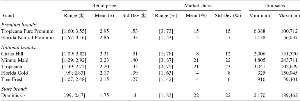
1, . . . ,89). Table 1 provides summary statistics pooled across the stores for average weekly prices, market shares, and unit sales of the brands.
As Table 1 reveals, the brands can be classified into three price-quality tiers: the premium brands (made from freshly squeezed oranges), the national brands (reconstituted from frozen orange juice concentrate), and the store brand (Do-minick’s private label brand). The differences in quality across the tiers are well represented by higher (lower) average prices for higher (lower) quality tier brands. Average weekly prices and market shares of all brands vary considerably, reflecting the frequent use of promotions.
We now illustrate the usefulness of imposing monotonicity constraints to estimate price response functions considering as example the brand Florida Gold. We focus on two distributional models, namely a lognormal model
salesst∼LN(ηst, σ2), (27)
Table 1. Descriptive statistics for weekly brand prices, market shares, and unit sales. Refrigerated orange juice category (64 oz)
Retail price Market share Unit sales
Brand Range ($) Mean ($) Std Dev ($) Range (%) Mean (%) Std Dev (%) Minimum Maximum
Premium brands:
Tropicana Pure Premium [1.60; 3.55] 2.95 .53 [3; 73] 15 15 6,388 100,712
Florida Natural Premium [1.57; 3.16] 2.86 .33 [1; 53] 5 7 1,138 56,037
National brands:
Citrus Hill [1.09; 2.82] 2.31 .31 [1; 78] 8 12 2,006 151,570
Minute Maid [1.29; 2.92] 2.23 .40 [3; 87] 21 22 4,805 243,711
Tropicana [1.49; 2.75] 2.20 .35 [2; 75] 21 23 3,041 102,629
Florida Gold [.99; 2.83] 2.17 .39 [1; 63] 4 8 325 150,945
Tree Fresh [1.07; 2.48] 2.15 .27 [1; 42] 4 6 916 39,401
Store brand:
Dominick’s [.99; 2.47] 1.75 .4 [1; 83] 22 22 2,170 189,462
which can be equivalently written in terms of the assumption of a Gaussian distribution for the natural logarithm of the response as
log(salesst)∼N(ηst, σ2), (28)
and a Gamma model
salesst∼G(exp(ηst), ν), (29)
wheresalesst denotes the unit sales of Florida Gold in stores
and weekt. Note that the exponential function is the so-called natural link function for a Gamma model. The scale parameter
ν is supplied with a Gamma prior with parametersaν=.001, bν=.001 and estimated in a Metropolis–Hastings step.
As mentioned above, the use of a lognormal model is the standard approach in marketing to relate brand sales to pro-motional instruments. The Gamma model, on the other hand, provides high flexibility with respect to the shape of the dis-tribution (e.g., it can take on a highly skewed disdis-tribution) and is used to demonstrate the applicability of our method in the non-Gaussian case. Like Kalyanam and Shively (1998) and van Heerde et al. (2001), we choose a semiparametric additive pre-dictor to model sales response, with nonparametric terms for own- and cross-price effects as well as weekly effects, and para-metric terms for own and competitive display and store-specific effects. According to economic theory and the empirical find-ings discussed in Section 3.1, we expect the unit sales of Florida Gold to be an antitonic function in own promotional price and an isotonic function in competitive items’ promotional prices rather than to show a nonmonotonic shape, respectively. Specif-ically, we estimate three variants of the semiparametric additive predictor for both the lognormal and the Gamma model:
η(st1)=f1RW_antitonic1 (pricest)+f2RW_isotonic1 (price_premiumst)
+f3RW_isotonic1 (price_nationalst)
+f4RW_isotonic1 (price_Dominicksst)+f5RW2(week)
+frandom(store)+γ1displayst+γ2display_premiumst
+γ3display_nationalst+γ4display_Dominicksst, (30) η(st2)=f1RW_antitonic2 (pricest)+f2RW_isotonic2 (price_premiumst)
+f3RW_isotonic2 (price_nationalst)
+f4RW_isotonic2 (price_Dominicksst)+f5RW2(week)
+frandom(store)+γ1displayst+γ2display_premiumst
+γ3display_nationalst+γ4display_Dominicksst, (31)
and
η(st3)=f1RW2(pricest)+f2RW2(price_premiumst)
+f3RW2(price_nationalst)
+f4RW2(price_Dominicksst)+f5RW2(week)
+frandom(store)+γ1displayst+γ2display_premiumst
+γ3display_nationalst+γ4display_Dominicksst. (32)
The three variants differ in the specification of the unknown smooth functionsf1–f4for own- and cross-price effects. These are estimated either by P-splines with monotonicity constraints, with first-order random walk prior (η(1)) or second-order ran-dom walk prior (η(2)), respectively, or by unconstrained P-splines with second-order random walk prior (η(3)) as a
ref-erence. The choice of the reference specification is based on a study conducted by Lang and Brezger (2004) who reported su-perior results for P-splines with second-order rather than first-order random walk priors in the unrestricted case.pricedenotes Florida Gold’s actual price in storesand weekt, anddisplay
is an indicator variable representing the usage (1) or nonusage (0) of an in-store display for Florida Gold in storesand week
t. Similarly to Blattberg and George (1991), we capture cross-price effects in a more parsimonious way through the use of competitive variables at the tier level rather than the individual brand level:price_premiumst andprice_nationalst indicate the
minimum price for competing brands within the premium brand and the national brand tier in storesand weekt, respectively, whereasprice_Dominicksst is the actual price of Dominick’s
private label brand in storesand weekt. It is important to note that the price of Florida Gold (which itself is a national brand) is excluded from computingprice_nationalst. Accordingly, the
indicator variables display_premiumst and display_nationalst
take the value ‘1’ if a display is used for at least one brand
within the respective tier in store sand week t, and ‘0’ oth-erwise.display_Dominicksst is the display dummy for the
pri-vate label brand indicating if Dominick’s supports its own brand with a display or not in storesand weekt.γ1toγ4denote the corresponding display effects to be estimated.
Theweekcovariate is incorporated to capture seasonal and missing variable (e.g., manufacturer advertising) effects, and the store covariate to accommodate differences in base sales of Florida Gold across the stores, for example, due to their spa-tial location. The effect ofweekis modeled as a P-spline with second-order random walk prior andst ore is incorporated as a random effect. We use cubic splines with 20 knots for all P-spline terms, except for theweekeffect, where we use 40 knots to be able to account for possibly strong time variability. The specification with 40 knots for the time effect, however, is still much less costly in terms of degrees of freedom lost than if we were to use weekly indicator variables. Finally, the hyper-parametersσ2 andν are supplied with inverse Gamma priors
σ2∼IG(.001, .001)andν∼IG(.001, .001), respectively, and are estimated simultaneously with the regression parameters. The resulting models are referred to as LN1–LN3 for the log-normal variants and G1–G3 for the Gamma model variants in the following. With regard to the sampling process, we store every 10th sample of a Markov chain of length 10,000 (after the burn-in period) to obtain 1,000 draws for each parameter and take the means as parameter estimates.
4.3 Model Evaluation and Interpretation of Results
We evaluate the different models in terms of the average mean squared error (AMSE) in validation samples (also cf. van Heerde et al. 2001). Specifically, we randomly split the data into nine equally sized subsets and performed ninefold cross-validation. For each subset, we fitted the respective model to the remaining eight subsets making up the estimation sample and calculated the squared prediction errors of the fitted model when applied to the observations in this holdout subset (Efron and Tibshirani 1998). LetNdenote the number of observations of the entire dataset, and k(n) the holdout subset containing observation n. Let further sales−nk(n) indicate the fitted value of observationncomputed from the estimation sample without subsetk(n); then the AMSE of prediction is
AMSE= 1
Because we are interested in unit sales rather than log unit sales of Florida Gold, conditional mean predictions from the esti-mated lognormal models were obtained as follows (Goldberger 1968; Greene 1997):
whereηniis the additive predictor for observationnand stored
iterationi, andσi2denotes the residual variance of the respec-tive lognormal model in iterationi. For the Gamma model, no correction factorσi2/2 is required for the conditional mean pre-dictions.
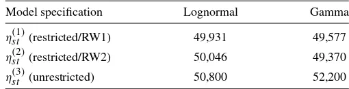
Table 2. Evaluation of models in terms of AMSE
Model specification Lognormal Gamma
ηst(1)(restricted/RW1) 49,931 49,577
ηst(2)(restricted/RW2) 50,046 49,370
ηst(3)(unrestricted) 50,800 52,200
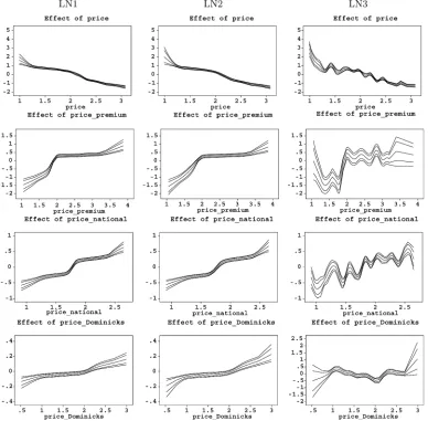
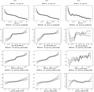
The validation results are displayed in Table 2. Under both the lognormal and the Gamma distribution, the models with monotonicity constraints (LN1, LN2, G1, G2) clearly outper-form the respective model without monotonicity constraints (LN3, G3). Interestingly, whereas in the unrestricted case the lognormal model (LN3) yields a smaller AMSE compared to the Gamma model (G3), the restricted Gamma models G1 and G2 provide the highest predictive validity. Furthermore, the dif-ferences between restricted models with first-order and second-order random walk priors for the nonparametric terms are virtu-ally negligible. These results indicate that imposing monotonic-ity constraints on own- and cross-item price effects can substan-tially improve the predictive validity of a sales response model. Figures 2 and 3 show the nonparametrically estimated own-and cross-price effects for Florida Gold resulting from the log-normal models (LN1–LN3) and the Gamma models (G1–G3), respectively. Shown are the posterior means as well as 80% and 95% pointwise credible intervals. To ensure identifiability, the functions are centered to have mean zero in every iteration of the MCMC procedure, that is, 1/range(xj)
fj(xj) dxj =0.
The subtracted means are added to an intercept term, which is not displayed here. It is important to note that, because to this centering, it is not necessary to explicitly restrictβ1 to be neg-ative andβ21, β31, β41to be positive to obtain monotonicity for the own- and cross-item price response curves. As can be seen, the effects are very similar for corresponding model versions (LN1|G1, LN2|G2, and LN3|G3), except for the own-price ef-fect which reveals a stronger increase in unit sales for very low prices under the Gamma distribution. Probably, this difference in own-price response is responsible for the higher predictive validity of the Gamma models. As already indicated by the AMSE values, there is also not much difference in own- and cross-price effects between the restricted Gamma models G1 and G2. We therefore focus in the following on Gamma model G2, the model with the highest predictive validity, for interpre-tation of results. Importantly, the unrestricted models LN3 and G3, which are inferior in predictive validity, show strong local nonmonotonicities in both own- and cross-price effects, which indicates too much flexibility (strong overfitting) of an uncon-strained estimation.
Our results are similar to the findings of van Heerde et al. (2001) with respect to the shape of price response functions. Specifically, the own-price response curve for Florida Gold shows a reverse S-shape with an additional increase in sales for extremely low prices. This strong sales spike can be attributed to an odd pricing effect at 99 cents, the lowest observed price of Florida Gold (cf. Table 1). The cross-price response curve with respect to the premium tier brands reveals a reverse L-shape and a threshold effect for competitive prices over two dollars. In other words, only if one of the premium brands is priced lower than two dollars, unit sales of Florida Gold significantly
Figure 2. Estimated curves for own-price (price) and tier-specific cross-price (price_premium,price_national,price_Dominicks) effects on unit sales of Florida Gold. Columns 1–3 show the effects for the models LN1–LN3. Shown are the posterior means as well as 80% and 95% pointwise credible intervals.
decrease and consumers switch up to the low-priced premium brand. The cross-price effect with respect to the national brand tier (the tier of Florida Gold) is S-shaped but by far less strong than the premium tier effect, which contradicts the hypothesis that brands which are priced closer to each other (like Florida Gold and the other national brands) are more competitive than brands priced farther apart (like Florida Gold and the premium brands). Finally, the cross-price effect of Dominick’s private la-bel brand on Florida Gold’s sales is almost negligible. Com-paring the three cross-price effects in magnitude, our results confirm previous empirical findings of asymmetric quality tier competition. Specifically, a price cut by a premium brand may draw substantial sales from Florida Gold, whereas a price cut by a private label brand does not. As expected, the own-price effect is much stronger than each of the cross-price effects.
Tables 3 and 4 provide parameter estimates for the display effects and the corresponding multiplier effects (Leeflang, Wit-tink, Wedel, and Naert 2000). The multiplier effects are ob-tained from the transformation
1 1,000
1,000
i=1
exp{γj i}, j=1, . . . ,4. (35)
Shown are the posterior means, posterior standard deviations, and the corresponding 2.5% and 97.5% quantiles, respectively. Multipliers with values larger (smaller) than 1 indicate a pos-itive (negative) effect on unit sales of Florida Gold. γ1i
de-notes the own display effect of Florida Gold, and γ2i to γ4i
refer to the tier-specific competitive display effects.i denotes theith stored sample for the respective parameter. Except for the cross-display effect of Dominick’s private label brand, the display multipliers show the expected impact. For example, if a display is used for Florida Gold, its unit sales increase on aver-age by a factor of 1.36, whereas a display for a premium brand causes a decrease in Florida Gold’s unit sales of about 11% on average. The display effect with respect to the brands in the na-tional tier (except Florida Gold) is not significant. One possible explanation for the positive cross display effect of Dominick’s private label could be that promotion activities of Dominick’s for its own store brand are especially distinct and stimulate not only own brand sales but also sales of some other brands in the category. As expected, the own display effect is much stronger than competitive display effects.
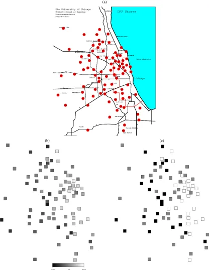
Finally, Figure 4 shows estimated results for the store-specific random effect. The store effect is portrayed with a
Figure 3. Estimated curves for own-price (price) and tier-specific cross-price (price_premium,price_national,price_Dominicks) effects on unit sales of Florida Gold. Columns 1–3 show the effects for the models G1–G3. Shown are the posterior means as well as 80% and 95% pointwise credible intervals.
tial map that represents the store locations of Dominick’s Finer Foods in the Chicago metropolitan area. There is a noticeable difference in base sales across stores, with an apparent drop from the coastline in the east, where we have a high concen-tration of stores, to the interior region in the west. We found (weak) positive correlations between the store effect and the percentage of the population under age 9 (.28) and the percent-age of households with three or more members (.24). Hence, one possible explanation for the east-west drop of base sales may be that more households with little children live in the east part of the Chicago area, and people buy more orange juice
Table 3. Estimation results (posterior means, standard deviations, and 95% credible intervals) for the display effects (Model G2)
Posterior 2.5%-
97.5%-Effect mean quantile quantile
γ1(display) .30 (.04) .24 .38
γ2(display_premium) −.12 (.04) −.19 −.05 γ3(display_national) −.02 (.05) −.11 .08 γ4(display_Dominicks) .07 (.03) .00 .14
there because they are concerned with their children’s health. We abstain from depicting the estimated effect for the time co-variateweek, because it does not reveal any seasonal pattern nor a trend.
5. REFINEMENTS
In this section we present some refinements of our methodol-ogy. The refinements are illustrated for the lognormal model, which is the standard approach in marketing to relate brand sales to price and promotional instruments (cf. Sec. 4.2). First,
Table 4. Estimation results (posterior means, standard deviations, and 95% credible intervals) for the display multiplier effects (Model G2)
Posterior 2.5%-
97.5%-Effect mean quantile quantile
γ1(display) 1.36 (.05) 1.27 1.45
γ2(display_premium) .89 (.03) .83 .95 γ3(display_national) .98 (.05) .90 1.08 γ4(display_Dominicks) 1.07 (.04) 1.00 1.15
(a)
(b) (c)
Figure 4. (a) Map of the Chicago metropolitan area with store locations of Dominick’s Finer Foods. (b) Estimated random effect ofstore
for the Gamma model (G2). (c) Posterior probabilities ofstore. White (black) indicates strictly positive (negative) 95% credible intervals, gray indicates that the 95% credible intervals contain zero.
we provide a relaxation of our procedure to enforce monotonic-ity on P-splines to encompass a more general class of monotone P-splines. Second, we perform a sensitivity analysis on the number and location of the knots with respect to the nonpara-metric price terms in our empirical application. Third, we apply our methodology to another brand (Dominick’s store brand) to validate our results obtained for Florida Gold. We also compare the predictive power of our semiparametric models to the
log-linear (or exponential) model, which is one of the most widely used parametric specifications to estimate price response.
5.1 Generalization of Conditions for Monotonicity
The conditions (10) we suggested in Section 2.2 for impos-ing monotonicity constraints on nonparametric terms are suffi-cient, but not necessary. We employed these conditions in each
iteration of our sampler by admitting only posterior draws for a spline coefficientβψ(t )that fall inside of the interval bounded by the current states of the adjacent spline coefficients βψ(t )−1
andβψ(t+−11)(cf. Sec. 3.1). This updating mechanism guarantees that the first derivative of the resulting spline is either positive or negative over its entire domain; hence the estimated curve becomes either isotonic or antitonic. There may be, however, values outside of the interval [βψ(t )−1; βψ(t−+11)] that would not have destroyed the monotonicity of the curve (if admitted). In other words, excluding these values is sufficient, but not neces-sary, for monotonicity. As a consequence, with conditions (10), we covered only the class of monotone P-splines that can be represented with an ordered set of basis function coefficients
βj1, βj2, . . . , βj .
To get a sense of how restrictive our class of monotone P-splines is, we relaxed our condition to encompass the class of all monotone P-splines. This can be accomplished by admit-ting a wider range of posterior draws forβψ(t ),ψ=1, . . . , ,
t =1, . . . , T, and rejecting them if and only if we obtain a wrong sign for the derivative of the spline somewhere. Forcubic
P-splines, as considered in this article, checking this new con-dition is simplified by utilizing the properties that (a) each basis function coefficient impacts function values over a domain of onlyl+1=4 interknot regions (cf. Fig. 1), (b) the first deriv-ative is continuous, and (c) the second derivderiv-ative is a piecewise linear curve. Implementation of the new rejection rule is carried out by verifying that the first derivative is positive (negative) at the borders of the four regions and also at the minimum (max-imum) of these regions. (We thank an anonymous referee for her/his valuable comments on this topic.)
Based on this relaxation, we estimated two new variants of our semiparametric additive predictor: with first-order random walk prior (η(4)) and with second-order random walk prior (η(5)). We included both new variants in the sensitivity analy-sis whose results are presented below. The new variants are re-ferred to asrestricted/RW1/Randrestricted/RW2/Rin the fol-lowing, withRindicating the relaxation.
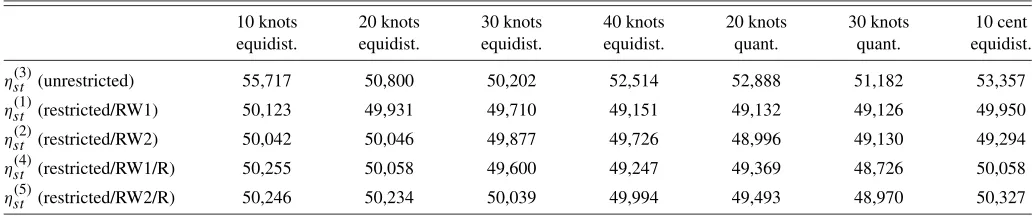
5.2 Sensitivity Analysis
To assess how strongly the predictive performance of our models is influenced by the number and location of knots used for the nonparametric price terms, we performed a sensitivity analysis. We estimated the five modelsη(1)–η(5) with (a) 10, 20, 30, and 40 equally spaced (equidistant) knots, (b) 20 and
30 knots positioned at the quantiles of the respective price co-variates, as well as (c) knots located at intervals of approxi-mately 10 cents within the price ranges. While alternatives (a) and (b) assume an equal number of knots across own- and cross-item price terms (implying unequal distances between each two knots for differently sized price ranges), alternative (c) instead leads to a different number of knots for price ranges of different span (but to equal distances between adjacent knots).
Table 5 shows the AMSE results of the sensitivity analysis, which can be summarized as follows: Independent of the num-ber and location of knots, the restricted models (η(1),η(2),η(4),
η(5)) are always superior in predictive validity to the respective unrestricted model. Specifically, the improvement in AMSE values from imposing monotonicity constraints is considerable for all four restricted model variants and by far greater than the corresponding differences in AMSE values between the re-stricted models, respectively. There is a tendency that models with first-order random walk prior (η(1)andη(4)) perform bet-ter than models with second-order random walk prior (η(2)and
η(5)). Furthermore, although the lowest AMSE value across all knot scenarios is associated with modelη(4) (48726; see col-umn30 knots quant.), modelsη(4)andη(5)perform worse than their counterparts η(1) and η(2) in almost all other cases, re-spectively. This is rather unexpected, sinceη(1) andη(2), rep-resenting the class of monotone P-splines constructable from an ordered set of basis function coefficients, occur as a spe-cial case of models η(4) andη(5) representing the class of all monotone P-splines. We therefore conclude that the conditions (10) for imposing monotonicity are not very restrictive, while at the same time requiring much more computational effort (i.e., CPU time).
There is also a tendency that the predictive performance of the restricted models slightly increases with more knots. Im-portantly, this latter finding did not hold for the Gamma mod-els (neither for the restricted variants nor for the unrestricted model) for which we also conducted a sensitivity analysis. We again, however, obtained a considerable improvement in predic-tive performance for all Gamma models with monotonicity con-straints compared to the unrestricted Gamma model under each of the seven knot scenarios. Based on these insights, the pre-diction improvement of the restricted models can be attributed to the monotonicity constraint rather than to the number and location of the knots.
Summarizing the main findings from our sensitivity analysis, there is evidence that the monotonicity constraint is the crucial part for the prediction improvement, rather than the number and location of the knots. Of course, more research with respect to
Table 5. Evaluation of lognormal models in terms of AMSE for Florida Gold
10 knots 20 knots 30 knots 40 knots 20 knots 30 knots 10 cent equidist. equidist. equidist. equidist. quant. quant. equidist.
η(st3)(unrestricted) 55,717 50,800 50,202 52,514 52,888 51,182 53,357
η(st1)(restricted/RW1) 50,123 49,931 49,710 49,151 49,132 49,126 49,950
η(st2)(restricted/RW2) 50,042 50,046 49,877 49,726 48,996 49,130 49,294
η(st4)(restricted/RW1/R) 50,255 50,058 49,600 49,247 49,369 48,726 50,058
η(st5)(restricted/RW2/R) 50,246 50,234 50,039 49,994 49,493 48,970 50,327
this point could be done, for example, by using a still larger number of knots or by estimating theoptimalnumber and lo-cation of knots. We leave these issues for future research. The results further indicate that the class of monotone P-splines rep-resentable with conditions (10) should not be very restrictive.
Finally, in contrast to our comparison with AMSE, we also computed the DIC upon the suggestion of one reviewer. This statistic favors the unrestricted models. The use of the DIC, however, has been considered critically as far as models with random effects are concerned (e.g., compare the discussion in Spiegelhalter, Best, Carlin, and van der Linde 2002). In our study, we have modeled the store effects by a random effect. We further regard cross-validation as a much stronger criterion to address our central question whether nonmonotonic effects indeed exist or rather represent an artifact: because model eval-uation is based on holdout sets not used for parameter estima-tion. Vehtari and Lampinen (2003) provided a similar argument in favor of cross-validation. They pointed out that information criteria ignore the uncertainty about parameter values.
5.3 Illustration for Dominick’s Store Brand
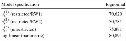
To validate our results obtained for Florida Gold, we replicate our application for Dominick’s, the retail chain’s own private label brand. Contrary to Florida Gold, which has been one of the brands with a rather low average market share (4%), Do-minick’s store brand has the highest market share (22%) on average in the product category (cf. Table 1). While the sales data indicated an out-of-stock situation for Dominick’s in two promotional weeks, we do not exclude these weeks from esti-mation and validation but instead use an additional dummy to account for this irregularity. Table 6 shows the AMSE results for the three modelsη(1),η(2), andη(3), where we use our de-fault choice of 20 equally spaced knots for all nonparametric price terms. Note that because Dominick’s is the only private label brand, we have only two cross-price effects included, one for the national brand tier and one for the premium brand tier.
The AMSE results for Dominick’s confirm our findings for Florida Gold that imposing monotonicity constraints on own-and cross-item price effects can improve the predictive validity of a sales response model. In particular, both restricted models
η(1) andη(2) perform much better than the unrestricted model
η(3), whereas the differences from using first-order or second-order random walk priors are almost negligible. Again, the es-timated curves for the unrestricted model showed strong local nonmonotonicities in both own- and cross-price effects, indicat-ing strong overfittindicat-ing. Also, as expected, the own-price effect of Dominick’s turned out to be much stronger than each of the two cross-price effects.
Table 6. Evaluation of models in terms of AMSE for Dominicks
Model specification lognormal
η(st1)(restricted/RW1) 70,620
η(st2)(restricted/RW2) 70,781
η(st3)(unrestricted) 75,881
log-linear (parametric) 80,891
To get a sense of how much we can gain from the nonpara-metric technique in general, we also estimated the log-linear model (or exponential model), which is one of the most widely used parametric models for problems as considered here. How-ever, to provide a fair comparison, we retained the cubic spline for the seasonal effect. The corresponding AMSE value pro-vided in Table 6 indicates that the log-linear model performs much worse compared to the nonparametric models. Whereas the unconstrained nonparametric model suffers from too much flexibility, the log-linear model now suffers from strong under-fitting.
6. DISCUSSION
We proposed a methodology to incorporate specific prior knowledge of a monotonic relationship between a response variable and one or more continuous covariates into (Bayesian) generalized additive models. Unlike other approaches to mono-tonic regression, our method offers the possibility of nonpara-metric monotonic modeling by penalized splines of arbitrary degree. Sampling is accomplished by block updates of nonpara-metric effects. An internal Gibbs sampler is employed for draw-ing random numbers from truncated multivariate normal densi-ties. Our approach can also accommodate additional covariates modeled by appropriate other specifications, such as parametric effects, unrestricted P-splines, random effects, or spatial effects as well as varying coefficient terms and interactions of covari-ates. We illustrated the methodology and its practical relevance in an empirical application estimating sales response for brands of refrigerated orange juice from store-level scanner data. Our results show that imposing monotonicity constraints for own-and cross-item price effects can considerably improve the pre-dictive validity of a sales response model. The methodology is implemented in the public domain software packageBayesX.
ACKNOWLEDGMENTS
This research has been financially supported in part by grants from the German Science Foundation (DFG), Sonder-forschungsbereich 386 “Statistical Analysis of Discrete Struc-tures.” We thank Ludwig Fahrmeir, Harald Hruschka, and Ste-fan Lang for helpful discussion. The data were provided by the James M. Kilts Center, GSB, University of Chicago.
APPENDIX A: B–SPLINE BASIS FUNCTIONS
The following results were obtained from De Boor (2001). A B-spline basis function of degreelwith equally spaced knots and distancehbetween each two adjacent knots can be written in terms of
Bψl(x)=(−1)l+1l+1t (x, ζψ)/(hll!), (36)
where l+1 is the difference operator of order l +1 and
t (x, ζψ)=(x−ζψ)l ifx > ζψ andt (x, ζψ)=0 otherwise.
B-spline basis functions of degree l with equally spaced knots with distancehcan be derived recursively starting from the corresponding B-spline basis function of degree 0:
Bψ0(x)=
Explicit formulas can also be derived. For example, for a cubic B-spline basis function (i.e.,l=3), we obtain
Bψ3(x)= 1 One fundamental property of a B-spline basis function is
Bψl (x) >0 for x ∈ ]ζψ−l−1, ζψ[ and Bψl (x)=0 otherwise.
A corresponding recursion formula for first-order derivatives is given byBψl′(x)=1h(Bψl−1(x)−Bψl−1
+1(x)).
APPENDIX B: CONDITIONS FOR MONOTONICITY
Letf (x)= ψ=1βψBψ(x), where Bψ(x), ψ=1, . . . , ,
denotes B-spline basis functions of a certain degree. To ensure that f′(x)≥0 or f′(x)≤0, it is sufficient to guarantee that subsequent parameters are ordered, such that
β1≤ · · · ≤β or β1≥ · · · ≥β , (40)
respectively.
Proof. We exploit the recursion formula for derivatives of B-splines and the fact that B-spline functions are nonnegative on their domain (see App. A).
Letting the superscriptl−1 denote basis functions of degree
l−1, we can writef′(x)in terms of
wherehdenotes the distance between two adjacent knots. The second equivalence in (41) holds, becauseB1l−1(x)=0 forx∈
[Received May 2004. Revised July 2006.]
REFERENCES
Allenby, G. M., Arora, N., and Ginter, J. L. (1995), “Incorporating Prior Knowl-edge Into the Analysis of Conjoint Studies,”Journal of Marketing Research, 32, 152–162.
Allenby, G. M., and Rossi, P. E. (1991), “Quality Perceptions and Asymmetric Switching Between Brands,”Marketing Science, 10, 185–204.
Bemmaor, A. C., and Mouchoux, D. (1991), “Measuring the Short-Term Effect of In-Store Promotion and Retail Advertising on Brand Sales: A Factorial Experiment,”Journal of Marketing Research, 28, 202–214.
Berger, J. O., and Pericchi, L. R. (2001), “Objective Bayesian Methods for Model Selection: Introduction and Comparison,” inModel Selection, Insti-tute of Mathematical Statistics Lecture Notes—Monograph Series, Vol. 38, ed. P. Lahiri, pp. 135–207.
Biller, C. (2000), “Adaptive Bayesian Regression Splines in Semiparametric Generalized Linear Models,”Journal of Computational and Graphical Sta-tistics, 9, 122–140.
Biller, C., and Fahrmeir, L. (2001), “Bayesian Varying-Coefficient Models Us-ing Adaptive Regression Splines,”Statistical Modeling, 2, 195–211. Blattberg, R. C., Briesch, R., and Fox, E. J. (1995), “How Promotions Work,”
Marketing Science, 14 (Part 2), G122–G132.
Blattberg, R. C., and George, E. I. (1991), “Shrinkage Estimation of Price and Promotional Elasticities,”Journal of the American Statistical Association, 86, 304–315.
Blattberg, R. C., and Neslin, S. A. (1990),Sales Promotion: Concepts, Methods, and Strategies, Englewood Cliffs, NJ: Prentice-Hall.
Blattberg, R. C., and Wisniewski, K. J. (1987), “How Retail Price Promotions Work,” Marketing Working Paper 42, University of Chicago.
(1989), “Price-Induced Patterns of Competition,”Marketing Science, 8, 291–309.
Brezger, A., Kneib, T., and Lang, S. (2005), “BayesX: Analysing Bayesian Structured Additive Regression Models,” Journal of Statistical Soft-ware, 14(11). Open domain software available from http://www.stat.uni-muenchen.de/˜bayesx/.
Brezger, A., and Lang, S. (2005), “Generalized Structured Additive Regression Based on Bayesian P–Splines,”Computational Statistics and Data Analysis, 50, 967–991.
Chen, M. H., and Dey, D. K. (2000), “Bayesian Analysis for Correlated Ordi-nal Data Models,” inGeneralized Linear Models: A Bayesian Perspective, eds. D. K. Dey, S. K. Ghosh, and B. K. Mallick, New York: Marcel Dekker, pp. 133–158.
De Boor, C. (2001),A Practical Guide to Splines(rev. ed.), New York: Springer. Denison, D. G. T., Mallick, B. K., and Smith, A. F. M. (1998), “Automatic Bayesian Curve Fitting,”Journal of the Royal Statistical Society, Ser. B, 60, 333–350.
Di Matteo, I., Genovese, C. R., and Kass, R. E. (2001), “Bayesian Curve-Fitting With Free-Knot Splines,”Biometrika, 88, 1055–1071.
Dunson, D. B., and Neelon, B. (2003), “Bayesian Inference on Order Constrained Parameters in Generalized Linear Models,” Biometrics, 59, 286–295.
Efron, B., and Tibshirani, R. J. (1998),An Introduction to the Bootstrap, Boca Raton, FL: Chapman and Hall/CRC.
Eilers, P. H. C., and Marx, B. D. (1996), “Flexible Smoothing Using B–Splines and Penalized Likelihood” (with comments and rejoinder),Statistical Sci-ence, 11, 89–121.
(2004), “Splines, Knots and Penalties,” technical report, available at http://www.stat.lsu.edu/bmarx/.
Fahrmeir, L., and Lang, S. (2001a), “Bayesian Inference for Generalized Addi-tive Mixed Models Based on Markov Random Field Priors,”Journal of the Royal Statistical Society, Ser. C, 50, 201–220.
(2001b), “Bayesian Semiparametric Regression Analysis of Multicate-gorical Time–Space Data,”Annals of the Institute of Statistical Mathematics, 53, 10–30.
Fahrmeir, L., and Tutz, G. (2001),Multivariate Statistical Modelling Based on Generalized Linear Models, New York: Springer.
Fan, J., and Gijbels, I. (1996),Local Polynomial Modelling and Its Applica-tions, London: Chapman and Hall.
Foekens, E. W., Leeflang, P. S. H., and Wittink, D. R. (1999), “Varying Pa-rameter Models to Accommodate Dynamic Promotion Effects,”Journal of Econometrics, 89, 249–268.
Friedman, J. H. (1991), “Multivariate Adaptive Regression Splines” (with dis-cussion),The Annals of Statistics, 19, 1–141.
Friedman, J. H., and Silverman, B. L. (1989), “Flexible Parsimonious Smooth-ing and Additive ModelSmooth-ing” (with discussion),Technometrics, 31, 3–39. Gamerman, D. (1997), “Efficient Sampling From the Posterior Distribution in
Generalized Linear Models,”Statistics and Computing, 7, 57–68.
Geweke, J. (1991), “Efficient Simulation From the Multivariate Normal and Student-tDistribution Subject to Linear Constraints,” inComputing Science and Statistics: Proceedings of the Twenty-Third Symposium on the Interface, pp. 571–578.
Goldberger, A. (1968), “The Interpretation and Estimation of Cobb–Douglas Functions,”Econometrica, 35, 464–472.
Greene, W. (1997),Econometric Analysis, Englewood Cliffs, NJ: Prentice-Hall. Gupta, S., and Cooper, L. (1992), “The Discounting of Discounts and
Promo-tion Thresholds,”Journal of Consumer Research, 19, 401–411.
Hansen, M. H., and Kooperberg, C. (2002), “Spline Adaptation in Extended Linear Models,”Statistical Science, 17, 2–51.
Hanssens, D. M., Parsons, L. J., and Schultz, R. L. (2001),Market Response Models: Econometric and Time Series Analysis, London: Chapman and Hall. Hastie, T., and Tibshirani, R. (1990),Generalized Additive Models, London:
Chapman and Hall.
(2000), “Bayesian Backfitting,”Statistical Science, 15, 193–223. Holmes, C. C., and Heard, N. A. (2003), “Generalized Monotonic Regression
Using Random Change Points,”Statistics in Medicine, 22, 623–638. Kalyanam, K., and Shively, T. S. (1998), “Estimating Irregular Pricing Effects:
A Stochastic Spline Regression Approach,”Journal of Marketing Research, 35, 16–29.
Kopalle, P. K., Mela, C. F., and Marsh, L. (1999), “The Dynamic Effect of Dis-counting on Sales: Empirical Analysis and Normative Pricing Implications,” Marketing Science, 18, 317–332.
Lang, S., and Brezger, A. (2004), “Bayesian P–Splines,”Journal of Computa-tional and Graphical Statistics, 13, 183–212.
Leeflang, P. S. H., Wittink, D. R., Wedel, M., and Naert, P. A. (2000),Building Models for Marketing Decisions, Boston: Kluwer Academic Publishers. Marx, B. D., and Eilers, P. H. C. (1998), “Direct Generalized Additive Modeling
With Penalized Likelihood,”Computational Statistics and Data Analysis, 28, 193–209.
Montgomery, A. L. (1997), “Creating Micro-Marketing Pricing Strategies Us-ing Supermarket Scanner Data,”Marketing Science, 16, 315–337. Mulherne, F. J., and Leone, R. P. (1991), “Implicit Price Bundling of Retail
Products: A Multiproduct Approach to Maximizing Store Profitability,” Jour-nal of Marketing, 55, 63–76.
Ramsay, J. O. (1988), “Monotone Regression Splines in Action,”Statistical Science, 3, 425–441.
(1998), “Estimating Smooth Monotone Functions,” Journal of the Royal Statistical Society, Ser. B, 60, 365–375.
Rao, V. (1993), “Pricing Models in Marketing,” inHandbooks in Operations Research and Management Science, Vol. 5, eds. J. Eliashberg and G. L. Lilien, Amsterdam: Elsevier, pp. 517–552.
Rue, H. (2001), “Fast Sampling of Gaussian Markov Random Fields With Ap-plications,”Journal of the Royal Statistical Society, Ser. B, 63, 325–338.
Robert, C. P. (1995), “Simulation of Truncated Normal Variables,”Statistics and Computing, 5, 121–125.
Salanti, G., and Ulm, K. (2003), “The Analysis of Dose-Response Relation-ship for Binary Data Using Monotonic Regression,”American Journal of Epidemiology, 157, 273–291.
Sethuraman, R., Srinivasan, V., and Kim, D. (1999), “Asymmetric and Neigh-borhood Cross-Price Effects: Some Empirical Generalizations,”Marketing Science, 18, 23–41.
Sivakumar, K., and Raj, S. P. (1997), “Quality Tier Competition: How Price Change Influences Brand Choice and Category Choice,”Journal of Market-ing, 61, 71–84.
Smith, M., and Kohn, R. (1996), “Nonparametric Regression Using Bayesian Variable Selection,”Journal of Econometrics, 75, 317–343.
Spiegelhalter, D. J., Best, N. G., Carlin, B. P., and van der Linde, A. (2002), “Bayesian Measures of Model Complexity and Fit” (with discussion), Jour-nal of the Royal Statistical Society, Ser. B, 64, 583–639.
Stone, C. J., Hansen, M., Kooperberg, C., and Truong, Y. K. (1997), “Polyno-mial Splines and Their Tensor Products in Extended Linear Modeling” (with discussion),The Annals of Statistics, 25, 1371–1470.
Tellis, G. J. (1988), “The Price-Elasticity of Selective Demand,”Journal of Marketing Research, 25, 331–341.
Ulm, K., and Salanti, G. (2003), “Estimation of General Threshold Limit Values for Dust,”International Archives of Occupational Environmental Health, 76, 233–240.
van Heerde, H. J., Leeflang, P. S. H., and Wittink, D. R. (2001), “Semipara-metric Analysis to Estimate the Deal Effect Curve,”Journal of Marketing Research, 38, 197–215.
(2002), “How Promotions Work: SCAN*PRO-Based Evolutionary Model Building,”Schmalenbach Business Review, 54, 198–220.
Vehtari, A., and Lampinen, J. (2003), “Expected Utility Estimation via Cross-Validation,” inBayesian Statistics, Vol. 7, eds. J. M. Bernardo, M. J. Bayarri, et al., New York: Oxford University Press, pp. 701–710.
Wahba, G. (1978), “Improper Priors, Spline Smoothing and the Problem of Guarding Against Model Errors in Regression,”Journal of the Royal Statis-tical Society, Ser. B, 40, 364–372.
Wilkinson, J. B., Mason, J. B., and Paksoy, C. H. (1982), “Assessing the Im-pact of Short-Term Supermarket Strategy Variables,”Journal of Marketing Research, 19, 72–86.
Wisniewski, K. J., and Blattberg, R. C. (1983), “Response Function Estima-tion Using UPC Scanner Data,” inProceedings of ORSA–TIMS Marketing Science Conference, ed. F. S. Zufryden, pp. 300–311.
Wong, C. M., and Kohn, R. (1996), “A Bayesian Approach to Additive Semi-parametric Regression,”Journal of Econometrics, 74, 209–235.
![Figure 1. B-spline basis functions of degree 3 covering the interval [A,B].](https://thumb-ap.123doks.com/thumbv2/123dok/1110265.759168/3.594.106.506.553.728/figure-b-spline-basis-functions-degree-covering-interval.webp)