Manajemen | Fakultas Ekonomi Universitas Maritim Raja Ali Haji 073500102288618775

(1)

Full Terms & Conditions of access and use can be found at

http://www.tandfonline.com/action/journalInformation?journalCode=ubes20

Download by: [Universitas Maritim Raja Ali Haji] Date: 13 January 2016, At: 00:38

Journal of Business & Economic Statistics

ISSN: 0735-0015 (Print) 1537-2707 (Online) Journal homepage: http://www.tandfonline.com/loi/ubes20

Bayesian Modeling and Computations in

Final-Offer Arbitration

Tim Swartz

To cite this article: Tim Swartz (2003) Bayesian Modeling and Computations in Final-Offer Arbitration, Journal of Business & Economic Statistics, 21:1, 74-79, DOI: 10.1198/073500102288618775

To link to this article: http://dx.doi.org/10.1198/073500102288618775

Published online: 01 Jan 2012.

Submit your article to this journal

Article views: 36

(2)

Bayesian Modeling and Computations in

Final-Offer Arbitration

Tim

Swartz

Department of Statistics and Actuarial Science, Simon Fraser University, Burnaby, BC, Canada V5A 1S6 (tim@cs.sfu.ca)

This article develops a Bayesian model for the analysis of bidding behavior in nal-offer arbitration. Posterior calculations are obtained using a Markov chain algorithm. An example is considered using salary data from Major League Baseball.

KEY WORDS: Latent variable; Major League Baseball; Markov chain Monte Carlo.

1. INTRODUCTION

In an attempt to curtail prolonged disputes and to avoid employee strikes, arbitration procedures are now common-place in many labor contracts.

Final-offer arbitration (FOA) is one such arbitration pro-cess whereby an employer offers a wage (or some other quan-tity)x, the employee independently requestsz, and an arbi-trator makes a decision by choosing either x or z (Stevens 1966). In conventional arbitration, the arbitrator is not con-strained to choosingxorz. The motivation behind FOA over conventional arbitration is to reduce the “chilling” effect; that is, knowing that either x or z will be chosen, negotiating teams ought to bargain more realistically and hence reduce the need for arbitration. Milner (1993) compared FOA with conventional arbitration on the basis of dispute deterrence. Ashenfelter, Currie, Farber, and Spiegel (1992) provided lab-oratory evidence that FOA does not reduce the chilling effect. In FOA theory, it is commonly assumed that the arbitra-tor behaves according to the parity concept (Farber 1980; Dworkin 1981). Under the parity concept, the arbitrator weighs the evidence and determines an undisclosed “fair” wage y. The arbitrator then chooses eitherxor z, depending on which value is closer toy. Typically,x < y < z.

Assuming parity, an active area of research concerns the behavior of the arbitrator. For example, one approach (Dworkin 1981; Fizel 1996) is based on probit models where the arbitrator’s decision is regressed against a set of covariates, including4zƒy5ƒ4yƒx5. However, a difculty associated with such models is that the unknownymust be estimated and this estimation is unaccounted for in the regression. Faurot and McAllister (1992) also considered arbitrator behavior where it is assumed thaty is normally distributed, offers are optimally risk neutral, and arbitrators are exchangeable.

In this article, I consider a related problem. I develop a model that focuses on the behavior of the bidders, that is, a model concerned with covariates that affect the bidsxandz. One approach is to regress the “standardized gap”4zƒx5=x or some transformed value against a set of covariates as in Frederick, Kaempfer, Ross, and Wobbekind (1996) and Frederick, Kaempfer, and Wobbekind (1992). A difculty with such an approach is that various information is intertwined in the standardized gap. For example, if large gaps are observed for female employees, it could be the case that employers dis-criminate against women. However, it could also be the case

that females have a higher sense of self-worth or that they are less risk averse than males.

In Section 2, I propose a Bayesian model that investigates the behavior of bidders. I dene variables related to the stan-dardized gap which help identify three quantities: (1) the mean amount by which the employer (employee) underestimates (overestimates) the fair wage, (2) the amount due to discrimi-nation on the part of the employer, and (3) the amount due to the misevaluation of self-worth on the part of the employee. These three quantities are all relative to the valueydetermined by the arbitrator. In addition, this model assumes the parity condition and takes into account the fact that y is unknown. In Section 3, the posterior calculations for this model are obtained using a Markov chain algorithm. Inference can thus be carried out for any function of the unknown parameters. Section 4 presents an example based on FOA data arising from Major League Baseball. Section 5 concludes with a short discussion.

2. A MODEL FOR FINAL–OFFER ARBITRATION

For ease of presentation, I initially consider a single arbi-tration case and omit subscripts. Let xdenote the employer’s offer and letzdenote the employee’s request. The “true” mar-ket value as determined by the arbitrator is a latent (i.e., unob-served) variable, which is denoted by y. The arbitrator now chooses eitherxorz. Under the parity concept (Farber 1980; Dworkin 1981), the arbitrator’s decision is given by

dD (

1 ifxis chosen (i.e.,yƒx < zƒy)1

0 ifzis chosen (i.e.,yƒx > zƒy)0 (1)

The data therefore consist ofx1 z, andd, where typicallyx < z. Note that in Major League Baseball salary arbitration, should x¶z, the FOA protocol is to inform the parties and abandon the arbitration hearing.

Consider a model where, conditional on 4y1 1 ‚1‘11‘2,

w11 w25,

4yƒx5=y¹Normal4w₁01‘2 151

4zƒy5=y¹Normal4w₂0‚1‘2

251 (2)

©2003 American Statistical Association Journal of Business & Economic Statistics January 2003, Vol. 21, No. 1 DOI 10.1198/073500102288618775

74

(3)

Swartz: Bayesian Modeling in Final-Offer Arbitration 75

and the two distributions are independent. This model should be interpreted as an approximation as it does not impose the condition x < z. In addition, the model is not necessarily behavioral as the employer and employee do not observe the fair wage y. Here w_i2 4r_i15 is a covariate vector whose values may be thought to affect the bids in FOA. For exam-ple, the components ofw_imay include covariates such as the race, sex, age, and occupation of the employee. The unknown parameters in (2) are  2 4r₁151 ‚ 2 4r₂151‘₁, and‘₂. In most applications,w₁Dw₂ would be chosen as it is difcult to imagine criteria that would be important to one party but of absolutely no importance to the other in determining bids. However, for the sake of generality, the distinction involving w₁ andw₂ will be maintained here.

Of primary interest are the vector parametersand‚. Let-ting₁and‚₁denote the constant terms, consider the baseline case where the remainingriƒ1 covariates inwi are equal to

0. Theny₁ is the mean amount that the employer underesti-mates the arbitrator’s fair wagey. Similarly,y‚₁ is the mean amount that the employee overestimates the arbitrator’s fair wagey. The quantities1and‚1may be tactical as suggested

by the game theory literature or may simply represent what the employer and employee deem to be fair. Also of interest are _i, iD11 : : : 1 r₁, and ‚_i, iD11 : : : 1 r₂. For example, if _i>0, this implies that the employer discriminates accord-ing to theith covariate when compared against the baseline case. In other words, a smaller offer is made to employees for whom theith covariate inw exceeds 0. One may also be interested in quantities such as w0

1ƒw20‚ for an employee

with specied covariatesw₁ and w₂. For ifw0

1 > w20‚, then

the employee would have a better chance than the employer of winning the FOA decision.

Introducing vector notation for thenindependent cases and letting6A—B7denote the conditional “density” ofA givenB, one can obtain the posterior density

61‚1‘₁1‘₂1y—x1z1d1w₁1w₂7 /61‚1‘₁1‘₂1y1x1z1d—w₁1w₂7 D6d—1‚1‘11‘21y1x1z1w11w27

61‚1‘11‘21y1x1z—w11w27

D6d—y1x1z76z—1‚1‘₁1‘₂1y1x1w₁1w₂7

6x—1‚1‘₁1‘₂1y1w₁1w₂761‚1‘₁1‘₂1y—w₁1w₂7 D6d—y1x1z76z—‚1‘₂1y1w₂7

6x—1‘₁1y1w₁761‚1‘₁1‘₂76y71 (3) where it is assumed that41 ‚1‘₁1‘₂1 y5does not depend on w₁andw₂(relaxed in Section 4) and that the latent vectoryis independent of41 ‚1‘₁1‘₂5. Here6d—y1 x1 z7is a point mass according to the parity concept (1) and can be expressed as

n Y

iD1

diI4yiƒxi< ziƒyi5C41ƒdi5I4yiƒxi> ziƒyi51

whereI is the indicator function. The densities6z—‚1‘₂1 y7¹

Qn

iD1Normal4yiCw02i‚yi1‘22y 2

i5 and 6x —1‘11 y7¹

Qn

iD1

Normal4y ƒw0 _y_1‘2_y2₅ _{follow immediately from (2).}

For 61 ‚1‘11‘27, one can use the improper prior

den-sity 1=4‘₁‘₂5, which is a standard reference prior (Berger 1985). Finally, the modeling is complete by dening6y7/1. Although this is a standard reference prior, which is sensible given the application in Section 4, in other applications where good prior information is available, one might consider a sub-jective prior density for6y7. Note also that, although it causes neither inferential nor computational difculties, the posterior density (3) is not dened when any y_iD0, iD11 : : : 1 n. In the Appendix, it is shown that the posterior is proper.

The posterior density (3) is an4nCr1Cr2C25-dimensional

function which fully describes the uncertainty in the parame-ters given the data. However, in practice, one may be primarily interested in marginal posterior characteristics (e.g., expecta-tions with respect to and ‚). As the calculation of these characteristics involves intractable high-dimensional integrals, the characteristics are estimated using a Markov chain Monte Carlo algorithm in Section 3.

Note that a simplication of the model can be obtained by imposing the restriction‘ D‘₁D‘₂. In this case, the posterior density becomes

61 ‚1‘ 1 y—x1 z1 d7/6d—y1 x1 z76z—‚1‘ 1 y1 w₂7

6x—1‘ 1 y1 w₁761 ‚1‘ 76y71 (4) where 61 ‚1‘ 7 is given by the improper prior density 1=‘. In practice, one might begin with model (3), and if the pos-terior analysis shows‘₁º‘₂, then proceed with the more parsimonious model (4). Note also that model (3) can be viewed as a generalization of an ordinary regression model. For if the uncertainty in the latent variable y is reduced (i.e., y approaches a point mass at some known y

0), then

the posterior density converges to the density proportional to 6z—‚1‘₂1 y

01 w27 6x—1‘11 y01 w17 61 ‚1‘11‘27.

In passing, note that a classical likelihood analysis would involve only the rst three factors of the posterior density (3). The maximization of the log-likelihood would most con-veniently proceed by rst maximizing with respect to yD y41 ‚1‘₁1‘₂5 for which an analytic expression is avail-able. SubstitutingyD Oy41 ‚1‘₁1‘₂5into the log-likelihood, one could then numerically maximize with respect to 41 ‚1‘₁1‘₂5. An inferential difculty with maximum like-lihood concerns the increasing dimensionality of the param-eter space (i.e., nCr₁Cr₂C2) as the sample size grows and this argues against the use of standard asymptotic theory. In contrast, the Bayesian approach provides exact inferences from the posterior distribution and the Markov chain algo-rithm allows the investigation of any posterior characteristic of interest.

3. POSTERIOR CALCULATIONS VIA GIBBS SAMPLING

The Gibbs sampling algorithm (Geman and Geman 1984; Gelfand and Smith 1990) provides an iterative approach to simulation from a target distribution. In the current problem,

(4)

an implementation of Gibbs sampling proceeds by setting

repeating the following stepsMCN times:

4i5 generate4j5_¹£

The idea is to sample from the full conditional distributions in (i)–(v) until the vector ˆ4j5 _D₄4j5_{1 ‚}4j5_1‘4j5 terior distribution. Note that convergence to the posterior as M! ˆis a property of the Gibbs sampling algorithm. One can then average the variatesˆ4MC15_{1 : : : 1 ˆ}4N 5_{to estimate}

var-ious posterior characteristics.

To generate from the full conditional distribution of‘1,

one can generatev₁¹Gamma4n=21 k₁5, wherek₁DPn

iD14xiƒ

y_iCw0

1iyi52=42yi25, and then set ‘1D1=

p_v

1. Similarly, to

generate from the full conditional distribution of‘₂, one can generate v₂¹ Gamma4n=21 k₂5, where k₂ DPn

The derivation of the full conditional distribution for requires some algebra. For example,

6—¢7/exp

The remainingnfull conditional distributions are nonstan-dard as the density6yi—¢7is proportional to

g_i4y_i5D

where I denotes the indicator function. Rather than sample from (6) directly, one can “imbed” a Metropolis step by setting aiD4xiCzi5=2 and introducing the proposal densities

hi14y5D43=ai5exp834yƒai5=ai91 y < ai1

when diD1 and

hi04y5D43=ai5exp8ƒ34yƒai5=ai91 y > ai1

when diD0. The proposal densities are convenient as they

allow efcient variate generation via inversion. The proposal densities also capture the essential features of the g_i4y5 and therefore yield high acceptance rates. Note that the proposal densities have exponentially decreasing tails extending from the estimatea_iD4x_iCz_i5=2 of the true market valuey_i. The jth iteration of the Metropolis step (see Gilks, Richardson, and Spiegelhalter 1996) then proceeds by generating u¹

Unif40115, generatingy4j5_i ¹h_d

Therefore, the Markov chain Monte Carlo algorithm is eas-ily implemented and provides a methodology for studying the bidding behavior in FOA. Note that minor simplications arise in the algorithm when the posterior density (4) is considered.

4. ANALYSIS OF MAJOR LEAGUE BASEBALL SALARY DATA

Salary data were obtained based on 161 cases of FOA in Major League Baseball during the period 1990 through 2001. The covariate wDw₁Dw₂ is four dimensional (i.e., r₁Dr₂D4) where the rst coordinate is the constant term and the second coordinate is 1 (0) corresponding to a pitcher (non-pitcher). The third coordinate is a race variable given by 1 (0) for whites (non-whites) where the non-white setting refers to blacks and Latinos. Note that, although race is not scientically well dened, there was complete agreement and no indecisiveness in two independent assignments of the race variable by viewing photos of the 161 baseball players. The fourth coordinate is an age variable given by ageƒ22 where age is the player’s age at the time of arbitration.

(5)

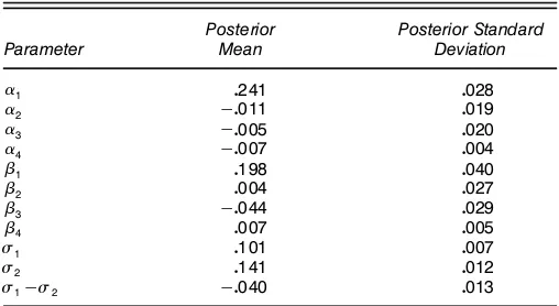
Table 1. Estimates of Posterior Means and Standard Deviations Based on Model (3)

Posterior Posterior Standard

Parameter Mean Deviation

₁ 0241 0028

2 ƒ0011 0019

3 ƒ0005 0020

4 ƒ0007 0004

‚1 0198 0040

‚2 0004 0027

‚3 ƒ0044 0029

‚4 0007 0005

‘1 0101 0007

‘₂ 0141 0012

‘1ƒ‘2 ƒ0040 0013

Table 1 provides estimates of the posterior means and stan-dard deviations of various parameters of interest based onND

105_{iterations of the Markov chain algorithm. The calculations}

require approximately 10 minutes of computation on a Sun workstation. Since‘O₂>‘O₁, one can conclude that players are more variable in their bids than owners. Also observe that there does not seem to be much of an effect due to position (pitcher/non-pitcher) as the bulk of the posterior distributions for 2 and‚2 are centered near 0. Interestingly, there is no

indication of race discrimination on the part of the owners (i.e., O₃º0), and there is mild evidence that white players are more risk averse than blacks and Latinos (i.e., ‚O₃<0). The latter nding disagrees with the conclusions discussed in Fizel (1996). It is also of interest to note that O₄<0 and

O

‚4>0. This implies that owners discriminate against older

players (i.e., offer less), whereas older players are less risk averse (i.e., request more). Perhaps owners devalue the limited future of older players, whereas older players want to be pri-marily rewarded for past performance. It should be noted that one must be cautious in assigning a behavioral interpretation to the results as the employer and employee do not observe the fair wagey.

Now consider the analysis of a more complex model which allows one to investigate the sensitivity of the analysis with respect to the prior specication. Expanding on (3) withwD w₁Dw₂ andrDr₁Dr₂, consider the posterior density

61 ‚1‘₁1‘₂1 ‹1 y—x1 z1 d1 w7

/6d—y1 x1 z76z—‚1‘₂1 y1 w76x—1‘₁1 y1 w7 61 ‚1‘₁1‘₂76y—‹1 w76‹70 (7) In motivating the new model, one might reason that if the gaps depend on the covariatew, then so mighty. In (7), it is assumed that the yi are conditionally independent. Introduce

‹ 2 4r15and set

6yi—‹1 w7¹Normal ¡

wi0‹1 4ka052

¢

1

where a₀D$2,000,000 represents a typical salary in Major League Baseball. Here, the prior mean of yi can be

inter-preted as a base salary‹ which is then perturbed according

Table 2. Estimates of Posterior Means and Standard Deviations Based on Model (7)

Posterior Posterior Standard

Parameter Mean Deviation

₁ 0237 0028

2 ƒ0013 0019

3 ƒ0004 0020

4 ƒ0007 0004

‚1 0203 0040

‚2 0007 0027

‚3 ƒ0045 0028

‚4 0007 0006

‘1 0103 0008

‘₂ 0139 0012

‘1ƒ‘2 ƒ0036 0013 ‹₁ 211070608 8630256 ‹2 ƒ8360505 3510106 ‹3 ƒ2360098 3820086 ‹4 ƒ650895 1190514

to the nonconstant covariates. The prior standard deviation of y_i can be interpreted as k typical salaries wherek is a speci-ed hyperparameter. The model specication is completed by assigning the standard reference prior6‹7/1.

Under model (7), there are only two changes in the Markov chain computations. First, a multiplicative factor (i.e., 6y_i— ‹1 w7) is introduced to the full conditional densities (6). Sec-ond, an extra step is added to the Gibbs sampling algo-rithm corresponding to the generation of ‹ from its full conditional distribution. It is not difcult to show that6‹—¢7¹

Normal4ƒ1 V 5, where V D 4ka₀52₄Pn

iD1wiw0i5ƒ1 and ƒ D

4Pn

iD1wiwi05ƒ14

Pn

iD1wiyi5. The results of the Major League

Baseball analysis based onkD1 are given in Table 2. There is close agreement with the results from the simpler model (i.e., Table 1), indicating that the FOA model is robust with respect to the prior specication ofy. Furthermore, note that ‹1 and ‹2 are the only important parameters in ‹. That is,

the arbitrator’s fair wage is centered about $2,107,000 and is adjusted downward for pitchers. On average, then, among those who have gone through the arbitration process, pitchers do not command as high a salary as position players. Finally, as might be expected, whenk is large (i.e.,kD10), the prior for y is quite at and the subsequent analysis produces the same results as in Table 1 to three decimal places.

5. CONCLUDING REMARKS

In FOA, the data consist solely of the arbitrator’s decision d, the employer’s offerx, and the employee’s requestz. With only such data, it is impossible to determine which of the three parties are acting in an unbiased fashion. For example, with all of the arbitration outcomes falling in the employer’s favor, it could be the case that the arbitrator is unfair and/or the employer is submitting high offers and/or the employee is submitting high requests. Therefore, in studying FOA data, certain assumptions need to be made.

Most of the literature in FOA tends to focus on the behav-ior of the arbitrator where, for example,y is estimated (Fizel

(6)

1996) or it is assumed that the employer and employee sub-mit offers according to rational game theory considerations (Faurot and McAllister 1992).

In this article, I focus on the behavior of the employer and employee relative to the arbitrator. This is a convenient per-spective as the assumptions are weak and it is often thought that the arbitrator is an unbiased but random decision maker (Ashenfelter 1987). In this case, the behavior of the employer and employee can be interpreted in terms of departures from a position of “fairness.” The major contribution of the article is the development of a Bayesian model and the associated computations to investigate such departures.

ACKNOWLEDGMENTS

This work was supported in part by a grant from the Nat-ural Sciences and Engineering Research Council of Canada. The author thanks James Dworkin, David Faurot, and Steve Gietschier for assistance in obtaining the data. The author also thanks the Associate Editor and a referee for helpful com-ments that led to an improvement in the manuscript.

APPENDIX: PROPRIETY OF THE POSTERIOR

In light of the improper prior density 61 ‚1‘11‘276y7/

1=4‘₁‘₂5, one can establish that the posterior (3) is proper by showing that the integral

ZZZZZ 1

Integrating rst with respect to , concentrate on the inner integral

using the notation from Section 3 and setting Q1 D4Iƒ

A₁4A₁A0

Returning to the original integral (A.1), one can establish that the posterior is proper if

Z

is nite. Working on the two inner integrals and recalling the norming constant of the inverse gamma distribution, the posterior is proper if

Z

is nite. First, one needs to check the singularities of the inte-grand in (A.2). SinceQ₁andQ₂are positive denite matrices, singularities only occur when any of they_iD0,iD11 : : : 1 n, and it is straightforward to show that the limit of the inte-grand is nite as one approaches the singularities provided that n > 4r₁Cr₂C45=2. Therefore, it is only a matter of investi-gating the tail behavior of (A.1), and sincet0

Q1tandt‚0Q2t‚

are both bounded in the tails, integrability follows.

To establish the existence of moments for ‘₁ and‘₂, the proof is modied by changing the norming constants in the inverse gamma distributions. To establish the existence of moments for and ‚, modify the proof using the known moments of the multivariate normal distribution.

[Received March 2000. Revised August 2001.]

REFERENCES

Ashenfelter, O. (1987), “A Model of Arbitrator Behavior,”American Eco-nomic Review, 77, 342–346.

Ashenfelter, O., Currie, J., Farber, H. S., and Spiegel, M. (1992), “An Exper-imental Comparison of Dispute Rates in Alternative Arbitration Systems,”

Econometrica, 60, 1407–1433.

Berger, J. O. (1985), Statistical Decision Theory and Bayesian Analysis, New York: Springer-Verlag.

Dworkin, J. B. (1981),Owners Versus Players: Baseball and Collective Bar-gaining, Boston: Auburn House.

Farber, H. S. (1980), “An Analysis of Final-Offer Arbitration,”Journal of Conict Resolution, 24, 683–705.

Faurot, D. J., and McAllister, S. (1992), “Salary Arbitration and Pre-arbitration Negotiation in Major League Baseball,” Industrial and Labor Relations Review, 45, 697–710.

Fizel, J. (1996), “Bias in Salary Arbitration: The Case of Major League Base-ball,”Applied Economics, 28, 255–265.

Frederick, D. M., Kaempfer, W. H., Ross, M. T., and Wobbekind, R. L. (1996), “Race, Risk and Repeated Arbitration,” in Baseball Economics: Current Issues, eds. J. Fizel, E. Gustafson, and L. Hadley, Westport, CT: Greenwood Press, pp. 129–141.

Frederick, D. M., Kaempfer, W. H., and Wobbekind, R. L. (1992), “Salary Arbitration as a Market Substitute,” inDiamonds Are Forever: The Business

(7)

of Baseball, ed. P. M. Sommers, Washington, DC: Brookings Institution, pp. 29–49.

Gelfand, A. E., and Smith, A. F. M. (1990), “Sampling Based Approaches to Calculating Marginal Densities,”Journal of the American Statistical Asso-ciation, 85, 398–409.

Geman, S., and Geman, D. (1984), “Stochastic Relaxation, Gibbs Distribu-tions and the Bayesian Restoration of Images,”IEEE Transactions on Pat-tern Analysis and Machine Intelligence, 6, 721–741.

Gilks, W. R., Richardson, S., and Spiegelhalter, D. J. (ed.) (1996),Markov Chain Monte Carlo in Practice, London: Chapman & Hall.

Milner, S. (1993), “Dispute Deterrence: Evidence on Final Offer Arbitration,” inNew Perspectives on Industrial Disputes, eds. D. Metcalf and S. Milner, New York: Routledge, pp. 133–159.

Stevens, C. M. (1966), “Is Compulsory Arbitration Compatible with Bargain-ing?”Industrial Relations, 5, 38–52.