Electronic Journal of Qualitative Theory of Differential Equations Proc. 8th Coll. QTDE, 2008, No. 161-14;
http://www.math.u-szeged.hu/ejqtde/
About stability on bounded domains of the
state space
Vladimir R˘asvan
Department of Automatic Control,
University of Craiova,
A.I.Cuza, 13, Craiova, RO-200585, Romania
e-mail: [email protected]
Abstract
Modern aircraft control systems contain the so-called rate limiter elements which are in fact incorporating the saturation function which is a bounded nonlinearity. In certain critical cases the so-called sector rotation - a standard procedure in absolute stability - leads to the fact that the sector conditions are broken outside a bounded domain. In order to apply standard results of the absolute stability theory there will be combined the results of the hyperstability theory with those arising from Liapunov function theory since existence of a Liapunov function is up to now the best way to estimate stability domains. At the same time the stability conditions will be expressed in the language of some frequency domain inequality as required by the conditions of the practical problem that generated the mathematical one.
AMS Classification: 93D10, 34D20, 34D23
Keywords: absolute stability, bounded state space domain, frequency domain inequality
This paper is in final form, has been submitted to the Proceedings of 8th
1
A motivating problem
A genuine contemporary challenge for both engineers and mathematicians is the problem of the so called PIO - P(ilot) I(n the loop) O(scillations) of mod-ern combat (but also civil) aircraft. Their mechanism which is better and better understood shows a self-sustained oscillation proneness of the feed-back system pilot-aircraft: there exist situations when, paradoxically, the pilot’s efforts to control the aircraft result in some kind of de-stabilizing that generates uncontrollable self-sustained oscillations. Today the aircraft spe-cialists consider three kinds of PIO that may be present in aircraft dynamics. Without discussing here their significance, we just mention that our paper deals with the theory of the so-called PIO-II: their defining conditions are characterized by the modeling assumption that all elements of the system are linear except the so-called rate limiters of the actuators.
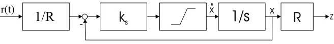
A. The rate limiter is an engineering structure that has to be modelled. The common structure is by now that of fig.1
1/R
k
s x1/s
xR
.
Z
-r(t)
Figure 1: Rate-limiter modeling
Let us consider a standard classical example arising apparently from air-craft control [2]
¨
y+ 2ζωny˙+ωn2y=−Kpy (1)
with 0 < ζ <1,Kp >0. Obviously this linear system is exponentially stable
for all Kp > 0; here Kp could be the equivalent pilot gain. But the pilot
command is usually applied through a rate limiter having the structure of fig.1 and this leads to a system of augmented dimension
¨
w+ 2ζωnw˙ +ωn2w=Kpz , z =Rξ
˙
ξ =sat(Ks(r/R−ξ)) , r =−w+v(t)
sat(e) = e
max {1,|e|}
The dimension augmentation limits Kp > 0 even in the linear case:
ap-plication of the Routh Hurwitz criterion for the linearized system
¨
w+ 2ζωnw˙ +ωn2w=KpRξ
˙
ξ =−Ksξ−
Ks
R (w−v(t))
(3)
will give
Kp <2ζωn(Ks+ 2ζωn+
ω2
n
Ks
) (4)
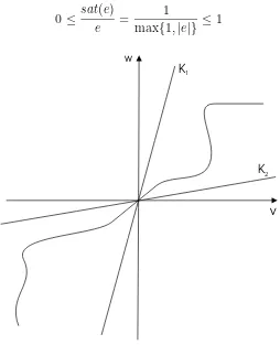
In the nonlinear case we have to remember that saturation is a nonlinear function confined to a sector (fig.2) namely (0,1]
0≤ sat(e)
e =
1
max{1,|e|} ≤1 (5)
w
K1
K2
v
Figure 2: Sector restricted nonlinear function
¨
This system corresponds to the critical case of a simple zero root in the absolute stability problem. If the Popov frequency domain inequality is used
1 +ℜe(1 +ıωβ)γ(ıω)≥0 (7)
where the transfer function γ(λ) reads here
γ(λ) =Ks
A tedious but straightforward computation will give the same inequality (4) as absolute stability condition; this means that (4) is a necessary and sufficient condition of absolute stability hence if Kp - the pilot gain in the
aircraft dynamics interpretation - is larger than the value prescribed by the RHS of (4), self sustained oscillations will occur - the PIO-II type.
B. We shall consider now a more recent version of aircraft dynamics -the longitudinal short period motion controlled by two actuators - -the elevon control and the canard control; we write down the model in deviations with the notations of the field
d
whereψ(σ) is the saturation function as previously. The characteristic equa-tion of the uncontrolled moequa-tion is
with Mq < 0, Mα > 0: we are in the case of the unstable aircraft which
displays a saddle point at the equilibrium - one of the eigenvalues is strictly positive.
Considering first the linearized case with ψ(σ) ≡ γσ, 0 < γ < 1 which has the characteristic equation
Pγ(λ)≡(λ+ωaγ)[λ3+ (ωaγ−Mq)λ2 + (ωaγA1−Mα)λ+ωaγA0] (11)
where we denoted: Mδ = Mδe+Mδc, A0 = Mδkα−Mα, A1 = Mδkq−Mq.
The (gain) Hurwitz condition will be
ωaγ > ξ+ =
A0+Mα+A1Mq+
p
(A0+Mα+A1Mq)2−4A1MqMα
2A1
(12)
This shows that the true stability sector (in the nonlinear case) has to be expected at most
ξ+
ωa
< ψ(σ) σ <1
In order to see the significance of this fact, introduce a new state variable - the elevon/canard unsymmetry
ζ = ∆e−∆c
to obtain the new system
d
dt∆α =q d
dt q=Mα∆α+Mqq+ (Mδe+Mδc)∆e−Mδcζ d
dt∆e =ωaψ(−kα∆α−kqq−∆e) dζ
dt =ωa[ψ(−kα∆α−kqq−∆e)−ψ(−kα∆α −kqq−∆e+ζ)]
(13)
d
dt∆α=q d
dt q =Mα∆α+Mqq+ (Mδe+Mδc)∆e d
dt∆e =ωaψ(−kα∆α−kqq−∆e)
(14)
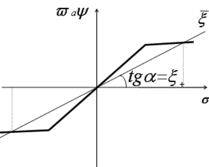
and will contain a single nonlinear element; the sector rotation
ϕ(σ) = −ξ+σ−ωaψ(−σ)
will give the system
d
dt∆α =q d
dt q=Mα∆α+Mqq+Mδ∆e d
dt∆e =−ξ+(kα∆α+kqq+ ∆e)−ϕ(kα∆α+kqq+ ∆e)
0< ϕ(σ)
σ < ωa−ξ+
(15)
One may see that the nonlinear function was confined to the sector with 0 as lower limit.
Figure 3: Sector rotation for saturation.
2
The mathematical problem and the main
result
We shall consider the following system
˙
x=Ax−bϕ(c∗x) (16)
with the usual notations of the absolute stability theory, whereϕ(σ) satisfies the sector condition
ϕ≤ ϕ(σ)
σ ≤ϕ¯ (17)
(see also fig.2 where the notations are slightly different) and assume that there exists some ϕ0 ∈[ϕ,ϕ¯] such that A−ϕ0bc∗ should be a Hurwitz matrix; this is some kind ofminimal stabilitysince if we want system (16) to be absolutely stable i.e. asymptotically stable for all functions satisfying (17) then we have to assume minimallythis stability for at least a single linear characteristic of the sector.
(ϕ(σ)−ϕσ)( ¯ϕσ−ϕ(σ))≥0 (18)
Moreover, ifσ(t) is some differentiable function on some interval, the deriva-tive being integrable on that interval, then we shall have
Z t
Consider now the linear controlled system
˙
x=Ax+bu(t) (21)
and associate to it the following integral index
η(0, t) = Z t
0
F(u(τ), x(τ))dτ (22)
where F(u, x) is the following quadratic form ofn+ 1 variables
F(u, x) = α0(u+ϕc∗x)(u+ ¯ϕc∗x) +
(23) + (α1(u+ϕc∗x)−α2(u+ ¯ϕc∗x))(c∗Ax+c∗bu)
and the integral index is defined for any pair of integrable vector valued functions. If, additionally x(t) and u(t) satisfy (21) then we may integrate by parts in (22) to obtain
η(0, t) = 1
G(u, x) = α0(u2+ (ϕ+ ¯ϕ)uc∗x+ϕϕ¯(c∗x)2) + (α1−α2)c∗(Ax+bu) (25)
Following V.M. Popov [4] we associate to the system defined by (21) and (24) the so-called system’s characteristic function χ:C×C7→C
χ(λ, σ) = 1 All functions are rational since they depend on the strictly proper rational function γ(σ) - the transfer function of the linear system defined by the controlled system (21) with the output ν =c∗x.
We shall consider now the positivity theory [4] - a generalization of the Yakubovich-Kalman-Popov Lemma - applied to the system defined by (21) and (24) with the characteristic function (26). If the frequency domain in-equality below holds
A small comment is necessary: if (27) holds for β ≥0 then we may take
The form (28) will turn to be useful in the construction of the suitable Liapunov function.
We shall make now use of the property of minimal stability in the sense of V.M. Popov [4]. Due to the existence of ϕ0 ∈ [ϕ,ϕ¯] such that A−ϕ0bc∗ is a Hurwitz matrix, we may chose in the system (16),(22)-(23) the control
u as
u(t) =−ϕ0c∗x(t) +ρ(t),
where x(t) = e(A−ϕ0bc∗)t
x0 and ρ(t) chosen according to [4], Chapter 5, in function of the various combinations of the free parameters αi ≥ 0 (as they
may follow from the fulfilment of the frequency domain inequality (27) for some α0 ≥ 0 and realβ) to obtain η(0, t)≤0. Therefore the matrix
P =H+1
2(α1ϕ−α2ϕ¯)cc
∗ (29)
results nonnegative definite. If additionally, (A, b) is a controllable pair then, as shown in (op. cit.), Chapter 4, we have even P a positive definite matrix for all combinations of the free parameters αi ≥0 (again, as they may follow
from the fulfilment of the frequency domain inequality (27) for some α0 ≥0 and real β). This fact will turn extremely useful in the following.
B. We shall return now to the nonlinear system (16) and make firstly a rather obvious but useful remark: let z(t) be some solution of (16) corre-sponding to some initial condition z(0) = x0; if we define u(t) =−ϕ(c∗z(t)) using this solution and apply it to (21), the solution x(t) of (21) defined by
x0 and u(t) will coincide with z(t).
Therefore we may consider the solutions of (16) as the solutions of (21) with the control input u(t) = −ϕ(c∗x(t)). We thus consider the integral
index (24) along the solutions of (21) with the control input defined as above. Taking into account (19) and (23) we find
η(0, t) = α1Ψ(ν(0))−α1Ψ(ν(t)) +α2Ψ(ν(0))−α2Ψ(ν(t)) +
(30)
+ α0
Z t
0
(ϕν(τ)−ϕ(ν(τ)))(ϕν(τ)−ϕ(ν(τ)))dτ
with ν = c∗x. We then equate (28) and (30) and use the notation (29) to
x∗(t)P x(t) +α
Introduce now the following state function that may be considered as a candidate Liapunov function
V(x) =x∗P x+α
1Ψ(c∗x) +α2Ψ(c∗x) (31)
If (20) and (29) are taken into account then one can see that
V(x) =x∗Hx+ (α
1−α2)
Z c∗x
0
ϕ(λ)dλ (32)
which is the standard Liapunov function “quadratic form plus integral of the nonlinear function” occurring in the absolute stability theory. The basic stability equality, which is written along the solutions of (16) becomes
V(x(t)) =V(x0) − α0
what shows that V is at least non-increasing along the trajectories of (16). We need now some information about the sign of V(x) itself. But V(x) is clearly positive definite since it has the form (31) hence V(x)≥x∗P x due
to the fact that αi ≥ 0, Ψ(ν) ≥ 0, Ψ(ν) ≥ 0. Since P > 0 as proved we
Liapunov function to be radially unbounded, the asymptotic stability will be global.
We may summarize the results proved above in the following
Theorem 1. Consider system (16) with ϕ : R 7→ R subject to inequalities
(17) assumed to be strict. If there exists ϕ0 ∈ (ϕ,ϕ¯) such that A−ϕ0bc∗
is a Hurwitz matrix and also the numbers α0 > 0 and β ∈ R such that the
frequency domain inequality (27) holds, then the equilibrium of (16) at the origin is globally asymptotically stable for all functions satisfying (17) with strict inequalities.
We observe, for the completeness of the results, that the sector conditions may be allowed to be non-strict provided the frequency domain inequality (27) is strict or system (16) has Adichotomic i.e. without eigenvalues on the imaginary axis. Details may be found in [4].
3
Application to the case of a bounded
domain in the state space
A. The motivating application showed that it is possible for the sector con-ditions to hold only in a bounded domain of the state space, of the form |c∗x| ≤ξ¯. Under these circumstances all development of the previous section
keeps its validity provided we remain in the state space domain defined by the above inequality. Consequently we need finding invariant subsets contained in|c∗x| ≤ξ¯. This is the reason why we took the Liapunov approach|c∗x| ≤ξ¯:
indeed, the easiest to recognize invariant sets of the system are those of the formV(x)≤cwherec >0 is some constant. Therefore the set of interest to our application would be
M= sup
c
{{x∈Rn : V(x)< c} ⊂ {x∈Rn : |c∗x|< σ0}} (34)
with V the Liapunov function of (32), H being the Hermitian matrix whose existence is ensured by the frequency domain inequality (27) and which may be determined by solving Linear Matrix Inequalities of Lurie type [1] and the
available MATLAB software. Observe that the supremum problem of (34)
The algorithm described above solves in a satisfactory way the mathe-matical problem issued from the practical one. The practical problem itself requires some other additional features among which the necessity to express the result in the language of those system parameters which may be mea-sured and evaluated by the customer (in the aircraft case - by the so called pilot ratings).
B. We turn to the equations of the aircraft application given by (15). The transfer function that is associated to the linear part of (15) is
ϑ(λ) = λ dition (27) will be read as a standard Popov inequality
1
ωa−ξ+
+ℜe(1 +ıωβ)ϑ(ıω)≥0 (36)
corresponding to the critical case of a pair of purely imaginary poles. The unique choice for β is as follows
¯
We may see that, in principle we may accept even infinitely large stability sectors since the second term in (37) is strictly positive for all ω ∈ R and,
And we thus arrive to the problem of the best Liapunov function. A rather general way of constructing it has been indicated above, involving theory and practice of Linear Matrix Inequalities. But, since the system is of low order, revisiting a classical book containing analytical methods for Liapunov functions construction in the problem of the absolute stability [3] might be rewarding.
References
[1] S. Boyd, L. El Ghaoui, E. Feron and V. Balakrishnan, Linear matrix inequalities in system and control theory, SIAM, Philadelphia, 1994.
[2] D. Graham and D. T. McRuer, Analysis of nonlinear control systems, J. Wiley,& Sons Inc., 1961.
[3] A.M. Letov,Stability of Nonlinear Controls(in Russian), Gostekhizdat, Moscow, 1955 (English version by Princeton Univ. Press, 1961); second edition, 1962 (English version, 1963)
[4] V. M. Popov, Hyperstability of Control Systems (in Romanian), Editura Academiei, Bucharest, 1966 (English version by Springer Verlag, 1973).