arXiv:1709.06006v1 [math.NT] 18 Sep 2017
FUNCTIONS ON A LOGARITHMIC SCALE
MARKUS FAULHUBER
Analysis Group, Department of Mathematical Sciences, NTNU Trondheim, Sentralbygg 2, Gløshaugen, Trondheim, Norway
Abstract. In this work we study and collect symmetry properties of the classical Jacobi theta functions. These properties concern the logarithmic derivatives of Jacobi’s theta func-tions on a logarithmic scale.
1. Introduction
Theta functions take a prominent role in several branches of mathematics. They appear in geometric function theory [1], [2], [3] the studies on energy minimization [4], the study of Riemann’s zeta and xi function [5], [8] or the theory of sphere packing and covering [7], including the recent breakthrough for sphere packings in dimension 8 by Viazovska [19] and in dimension 24 [6]. They also appear in the field of time-frequency analysis and the study of Gaussian Gabor frames [11], [12], [14] or the study of the heat kernel [16] to name just a few. The aim of this work is to reveal properties of the classical Jacobi theta functions looked at on a logarithmic scale as well as setting known results into a new context. We will encounter expressions of the form xff′((xx)), where f is at least continuously differentiable on R+ and possesses no zeros. Also, we will frequently use the differential operator xdxd and use the notation xdxdnfor its iterated repetition, i.e.,
x d dx
n
=x d dx
x d dx
n−1 .
In particular, we are interested in properties of the logarithmic derivative of a certain function f on a logarithmic scale. This statement should be interpreted as follows. By using the variable transformation y = log(x) we extend the domain from R+ to R and consider the new function log (f(ey)). Therefore, we get an extra exponential factor each time we take a (logarithmic) derivative. We have
d
dy log (f(e
y)) =eyf′(ey)
f(ey).
E-mail address: [email protected].
2010Mathematics Subject Classification. 26A51, 33E05.
Key words and phrases. Convexity, Jacobi Theta Function, Logarithmic Derivative, Logarithmic Scale.
The author was supported by the Austrian Science Fund (FWF): [J4100-N32] and [P27773-N23]. The computational results presented have been achieved (in part) using the Vienna Scientific Cluster (VSC).
By reversing the transformation of variables, we come back to the original scale, but the factor x stays. Without being explicitly mentioned, these methods were used in [11], [12], [15] to establish uniqueness results about extremal theta functions on lattices. This work provides a new point of view on as well as new results related to the mentioned articles.
Although we will mostly only consider real-valued functions in this work, we start by defining the theta function according to the textbook of Stein and Shakarchi [16].
Definition 1.1. Forz∈C andτ ∈H(the upper half plane) we define the theta function as
(1.1) Θ(z, τ) =X
k∈Z
eπik2τe2kπiz.
This function is an entire function with respect tozand holomorphic with respect toτ. As stated in [16], the function arises in many different fields of mathematics, such as the theory of elliptic functions, the theory of modular functions, as a fundamental solution of the heat equation on the torus as well as in the study of Riemann’s zeta function. Also, it is used to prove results in combinatorics and number theory.
The function can also be expressed as an infinite product.
Proposition 1.2 (Jacobi triple product). Forz∈Cand τ ∈H we have Θ(z, τ) =Y
k≥1
1−e2kπiτ 1 +e(2k−1)πiτe2πiz 1 +e(2k−1)πiτe−2πiz.
It also fulfills the following identity.
Theorem 1.3. For z∈C andτ ∈H we have
Θ z,−1τ= (−iτ)1/2eπiz2τΘ(τ z, τ).
For a proof of Theorem 1.3 and more details on theta functions of two complex variables as well as the product representation we refer to the textbook of Stein and Shakarchi [16].
Whereas derivatives of Θ with respect to z are often studied, it seems that studies of its derivatives with respect to τ are less common. The following Lemma contains a symmetry result for the logarithmic derivative of Θ with respect to τ.
Lemma 1.4. For z∈Cand τ ∈H we have
πiz2+τz ∂zΘ(τ z, τ) +∂τΘ(τ z, τ)
Θ(τ z, τ) −
1 τ
∂τΘ z,−τ1
Θ z,−1τ =− 1 2.
In particular, for z= 0 we get
τ∂τΘ(0, τ) Θ(0, τ) −
1 τ
∂τΘ 0,−1τ Θ 0,−1τ =−
1 2.
Proof. We start by taking the logarithm on both sides of the identity in Theorem 1.3 log Θ z,−τ1= 1
2log(−iτ) +πiz
2τ+ log (Θ(τ z, τ)).
Differentiating with respect to τ on both sides and a multiplication by τ yields, after
2. Jacobi’s Theta Functions
According to existing literature, we define the following functions which are usually denoted to Jacobi. We start with the following theta functions of two variables which we will then restrict to certain domains. For z∈C andτ ∈H we define
ϑ1(z, τ) =
X
k∈Z
(−1)(k−1/2)eπi(k−1/2)2τe(2k+1)πiz
= 2X
k∈N
(−1)(k−1/2)eπi(k−1/2)2τsin((2k+ 1)πz)
ϑ2(z, τ) =X
k∈Z
eπi(k−1/2)2τe(2k+1)πiz
= 2X
k∈N
eπi(k−1/2)2τcos((2k+ 1)πz)
ϑ3(z, τ) =X
k∈Z
e−πik2τe2kπiz
= 1 + 2X
k∈N
e−πik2τcos(2kπz)
ϑ4(z, τ) =X
k∈Z
(−1)ke−πik2τe2kπiz
= 1 + 2X
k∈N
(−1)ke−πik2τcos(2kπz).
We note that ϑ3(z, τ) = Θ(z, τ) and that any ϑj can be expressed via Θ from equation (1.1). The functions which we will study in the rest of this work are restrictions of the above functions with (z, τ) = (0, ix), x∈R+. In particular, all these functions are real–valued.
Definition 2.1 (Jacobi’s Theta Functions). For x ∈R+ we define Jacobi’s theta functions in the following way.
θ2(x) =ϑ2(0, ix) =
X
k∈Z
e−π(k−1/2)2x= 2X
k∈N
e−π(k−1/2)2x (2.1)
θ3(x) =ϑ3(0, ix) =X
k∈Z
e−πk2x = 1 + 2X
k∈N
e−πk2x (2.2)
θ4(x) =ϑ4(0, ix) =
X
k∈Z
(−1)ke−πk2x= 1 + 2X
k∈N
(−1)ke−πk2x (2.3)
All of the above functions can also be expressed by infinite products.
θ2(x) = 2e−
π
4x Y
k∈N
1−e2kπs 1 +e2kπs2
θ3(x) = Y
k∈N
1−e2kπs 1 +e(2k−1)πs2
θ4(x) =
Y
k∈N
1−e2kπs 1−e(2k−1)πs2
These representations can be quite useful when studying the logarithmic derivatives of these functions. We note that for z ∈R and purely imaginary τ =ix, x ∈R+ the theta function Θ(z, ix) is maximal forz∈Zand minimal forz∈Z+1
2. The first statement follows already from the definition of Θ whereas the latter argument can most easily be derived from the triple product representation. These special cases correspond to Jacobi’sθ3 and θ4 function
θ3(x) = Θ (0, ix)
θ4(x) = Θ 12, ix.
Forx∈R+, Jacobi’s θ2 function can be expressed via Θ in the following way.
θ2(x) =e−πx 4 Θ ix
2, ix
.
For what follows it is necessary to introduce the Fourier transform and Poisson’s summation formula which are given by
b
f(ω) =
Z
R
f(x)e−2πiωxdx, x, ω∈R
and
X
k∈Z
f(k+x) =X
l∈Z
b
f(l)e2πilx, x∈R.
respectively. Both formulas certainly hold for Schwartz functions and since we will apply both only on Gaussians we do not have to worry about more general properties for the formulas hold.
As a consequence of the Poisson summation formula we find the following, well-known identities
(2.4) √x θ3(x) =θ3 1x
(2.5) √x θ2(x) =θ4 x1 and √x θ4(x) =θ2 x1.
We note the common theme in the last identities which leads to the following lemma.
Lemma 2.2. Let r ∈ R and suppose that f, g ∈ C1(R+) do not possess zeros. If f and g satisfy the (generalized Jacobi) identity
then
Proof. Both, f and g are either positive or negative on R+ since they are real-valued, con-tinuous and do not contain zeros. As they also fulfill the identity xrf(x) = g 1x both of them possess the same sign. Without loss of generality we may therefore assume that both functions are positive because otherwise we change the sign which does not affect the results. Therefore, we have
log (xrf(x)) = log g x1.
Using the differential operator xdxd on both sides directly yields
r+xf
We remark that an alternative proof of Lemma 2.2 is given in [12] for the special case f = g = θ3 and r = 12 (a generalization of the proof in [12] is possible with the arguments given there). With this proof, the result
(2.6) xθ3′(x)
However, it seemed to have gone unnoticed that the result can be put into a more general context. With the previous lemma we also get the results
(2.7) xθ2′(x)
which were not given in [12]. All of the above results actually contain symmetry statements about logarithmic derivatives of Jacobi’s theta functions on a logarithmic scale. We note that the identities (2.6) and (2.7) are special cases of Lemma 1.4 when Θ is restricted to certain rays inC×H.
3. Properties of Theta-2 and Theta-4
We start with monotonicity properties of the logarithmic derivatives of Jacobi’s θ2 and θ4 functions on a logarithmic scale. The following result was already given in [12] and the proof can be established by using the product representation of θ4.
Proposition 3.1. The function xθ′4(x)
θ4(x) is strictly decreasing on
R+.
As a consequence of Proposition 3.1 we derive the following result.
Proposition 3.2. The Jacobi theta function θ4 is strictly logarithmically concave or, equiv-alently, θ′4(x)
θ4(x) is strictly decreasing. Also, the expression θ′
4(x)
Proof. The statement thatxθ′4(x)
and it follows that
0< x1θ
θ4(x) is strictly decreasing, hence, θ4 is logarithmically concave.
As a consequence of Proposition 3.1 and Lemma 2.2 we obtain the following property of θ2, which was already claimed, but not proven, in [12].
Proposition 3.3. The function xθ′2(x) or the first identity in (2.7) we obtain
d
In fact, Proposition 3.1 and Proposition 3.3 are equivalent by Lemma 2.2. In [12, Lemma 6.2] Proposition 3.3 was proved for x >1 by directly estimating xθ′2(x)
possess the same monotonicity properties.
Proposition 3.4. The Jacobi theta function θ2 is strictly logarithmically convex or, equiva-lently, θ′2(x)
θ2(x) is strictly increasing. Also, the expression θ′
2(x)
θ2(x) is negative.
Proof. The fact that θ2′(x)
θ2(x) <0 is easily checked by using (2.1). From the definition we see
that θ2 > 0 and due to its unconditional convergence, the derivatives can be computed by differentiating each term. We find out thatθ′
2(x)<0 and the negativity is proven.
The logarithmic convexity statement basically follows from the Cauchy-Schwarz inequality for the Hilbert–spaceℓ2(N). We compute
Strict logarithmic convexity of θ2 is now equivalent to
θ2′′(x)θ2(x)−θ2′(x)2 >0,
which can be re-written as
We set
θ4(x) is monotonically decreasing and convex. Both
properties were recently proved by Ernvall–Hyt¨onen and Vesalainen [9], [17]. We have a similar statement forθ2.
Proposition 3.5. The functions x2θ′2(x) Proof. The result involvingθ4 was proved by Ernvall–Hyt¨onen and Vesalainen [9].
We proceed with proving the result involvingθ2. We already know thatθ4is logarithmically concave, which is equivalent to the fact that θ′4(x)
θ4(x) is monotonically decreasing. By using
identity (2.7) we get
x2θ′2(x)
We note that a similar simple argument as used for the expression involving θ2 does not work forθ4. Due to identity (2.7) it also seems plausible to assume that for a monomial weight xr, the second power, i.e. x2, is the limit for the monotonicity properties of the logarithmic derivative ofθ2 andθ4 as stated in Proposition 3.5 and numerical investigations point in that direction.
Using the fact thatx2θ4′(x)
θ4(x) is strictly decreasing and Proposition 3.4 we conclude that
0< x2 d
Moreover, it seems to be true that x2dxd22 log(θ2(x)) is strictly decreasing, which would in
return imply that x2θ4′(x)
θ4(x) is strictly decreasing.
However, we leave this problem open and close this section with symmetry properties involving θ2,θ4 and repeated applications ofxdxd.
Proposition 3.6. For x∈R+ and 2≤n∈Nthe following holds.
4. Properties of Theta-3
In this section we will study properties of the logarithm of θ3 on a logarithmic scale as described in the introduction.
Proposition 4.1. The function xθ′3(x)
θ3(x) is strictly increasing on
R+.
This result was proved in [12]. As a consequence of Lemma 2.2 we get the following result which were already proved in the author’s doctoral thesis [10].
Proposition 4.2. For x∈R+ and 2≤n∈Nthe following holds.
x d dx
n
log (θ3(x)) = (−1)n
x d dx
n
log θ3 1x.
Proof. The statement is an obvious consequence of identity (2.6) and follows by induction.
The following statement and its proof were also already given in [10]. The techniques are similar to the techniques used by Montgomery in [15]. The computer algebra system Mathematica [20] was used at some points in the proof in order to compute explicit values or closed expressions for geometric series, but in principle all computations can also be checked by hand. The proof was adjusted to a level which should be quite accessible with no or only little help of computer algebra software.
Proposition 4.3. For x∈R+, the function
(4.1)
x d dx
3
log (θ3(x))
is positive for x∈(0,1) and negative forx >1. Also, the function is anti–symmetric in the following sense
x d dx
3
log (θ3(x)) =−
x d dx
3
log θ3 1x.
Proof. To simplify notation we set
ψ(x) = (log◦θ3)′(x) = θ3′(x) θ3(x).
Proposition 4.3 settles the part concerning the anti–symmetry of expression (4.1). Therefore, it is also clear that we only need to prove the statement about the negativity for x >1, the result forx∈(0,1) follows immediately. We start with the following calculation
(4.2)
x d dx
3
log (θ3(x)) =
x d dx
2
(x ψ(x))
=x ψ(x) + 3x2ψ′(x) +x3ψ′′(x).
In particular, Proposition 4.3 implies that ψ(1) + 3ψ′(1) +ψ′′(1) = 0. We proceed in two steps:
(i) We will show that xdxd3log (θ3(x)) is negative forx≥ 65.
First step: Sinceψis the logarithmic derivative ofθ3, we use Jacobi’s triple product formula forθ3 to obtain a series representation forψ. In order to control the expression in equation (4.2) we compute the derivatives of ψ up to order 2.
ψ(x) =X
we will have to work a bit more and estimate parts of the series by the leading term, by appropriate geometric series or by their values atx= 1 (or use combinations of the mentioned methods). We proceed with an upper bound for ψ′ forx >1.
ψ′(x) =X
With the same techniques we bound ψ′′ from above forx >1.
Therefore, we have forx >1
x d dx
3
log (θ3(x)) =x ψ(x) + 3x2ψ′(x) +x3ψ′′(x)
< 72x2−60x3e−πx.
It is quickly verified that 72x2−60x3 <0 forx > 65. In particular this shows that
x d dx
3
log (θ3(x))<0 forx > 6 5.
Second step: We will now show that xdxd3log (θ3(x)) is strictly decreasing at least on the interval 1,65. To do so, we apply the differential operatorxdxd on (4.1), i.e.,
x d dx
4
log (θ3(x)) =x d
dx x ψ(x) + 3x
2ψ′(x) +x3ψ′′(x)
=x ψ(x) + 7x2ψ′(x) + 6x3ψ′′(x) +x4ψ′′′(x).
In order to control the last expression for x >1, we need to estimate ψ′′′.
ψ′′′(x) =X
k≥1
−(2kπ)
4e−πkx e−5πkx+ 4e−3πkx+e−πkx
(1−e−2kπx)4
+2((2k−1)π)
4e−(2k−1)πx e−2(2k−1)πx
−4e−(2k−1)πx+ 1
1 +e−(2k−1)πx4
!
<−16π4e−πx(e−5π+ 4e−3π+e−π)
| {z }
>0.04
+ 2X
k≥1
((2k−1)π)4e−(2k−1)πx1 +e−(2k−1)πx−2
| {z }
<1
<−0.64π4e−πx+ 2π4e−πx+ 2X
k≥3
(kπ)4e−kπx
=−0.64π4e−πx+ 2π4e−πx 1−e−πx−5
| {z }
<1.25
×
1 + 16e−7πx
−79e−6πx+ 155e−5πx
−149e−4πx+ 81e−3πx
| {z }
<0.0065
<(2×1.259−0.64)π4e−πx
<183e−πx
Summing up the results, it follows that for x >1
x d dx
4
log (θ3(x)) =x ψ(x) + 7x2ψ′(x) + 6x3ψ′′(x) +ψ′′′(x)
It is quickly verified that 168x2−360x3+ 183x4e−πx <0 for x ∈1,60+2√46 61
. We note
that 60+261√46 >1.205.
By combining the two steps we see that the function xdxd3log (θ3(x)) is strictly decreasing at least on the interval (1,1.205) and negative forx >1.2. As the value at x= 1 is zero, we can finally conclude that the expression given in equation(4.1) is negative for x >1. Due to the already mentioned anti–symmetry with respect to the point (1,0) the function has to be
positive for 0< x <1.
The estimates in the proof are quite rough, but at the same time fine enough for the proof to work which is due to the rapid decay of the involved terms. Numerical inspections beforehand suggested that
x d dx
3
log (θ3(x))<0 forx >1.05.
and that
x d dx
4
log (θ3(x))<0 for 1< x <1.5.
We remark that the proof is quite sensible to the estimated constants and does for example not work if in the last step ψ′′′(x) is estimated by 184e−πx instead of 183e−πx.
Most recently, Vesalainen and Ernvall–Hyt¨onen [17], [18] proved Proposition 4.3 indepen-dently from this work. They used the result to prove a conjecture by Hernandez and Sethu-raman1 [13] (see also the references in [18]). The result by Vesalainen and Ernvall–Hyt¨onen (which the author was aware of) is an immediate consequence of Proposition 4.3 and reads as follows.
Theorem 4.4. For α, β∈R+ with 1≤α ≤β and x∈R+ we define the function
g(x) = θ3(βx)θ3(
x β)
θ3(αx)θ3(αx) .
Then
g(x) =g(1x)
and gassumes its global maximum only for s= 1. Also, the function is strictly increasing for s∈(0,1) and strictly decreasing for s∈(1,∞).
5. A Result Involving Theta-1
In contrast to the fact that ϑ1(0, τ) = 0 for all τ ∈ H, its derivative with respect to z evaluated at (0, ix), x∈R+ is not the zero function, in particular
(5.1)
∂zϑ1(0, ix) =X
k∈Z
(−1)k(2k+ 1)e−π(k+1/2)2x
= 2e−π4xY
k∈N
1−e−2kπx3, x∈R+.
1The author does not claim any credit for solving the conjecture by Hernandez and Sethuraman since the
The above function is often denoted byθ′
1(x), where the prime indicates differentiation with respect to z. The representation as infinite product is also well–known and follows from the Jacobi triple product representation of Θ (Proposition 1.2). Since the notation θ′
1 would be very misleading in this work we set
zθ1 =∂zϑ1(0, ix), x∈R+. Now we have the following identity (see e.g. [7, Chap. 4])
(5.2) θ2(x)θ3(x)θ4(x) =zθ1(x).
From this identity we derive the following result.
Proposition 5.1. For x∈R+, we define the function ψ1(x) =x3/4zθ1(x).
This function also has the following representations
ψ1(x) =x3/4 4
Y
j=2
θj(x) = 2x3/4e−π4xY
k∈N
1−e−2kπx3.
The function is positive and assumes its global maximum only forx= 1 andxψ′1(x)
ψ1(x) is strictly
decreasing. Furthermore,
ψ1(x) =ψ1(x1)
and, hence,
x d dx
n
ψ1(x) = (−1)n
x d dx
n
ψ1(1x), n∈N.
Proof. The different representations of ψ1 follow immediately from (5.1) and (5.2). It is obvious from the product representation thatψ1is positive. The symmetry ofψ1follows easily from (2.4) and (2.5). The (anti–)symmetry for the repeated application of the differential operator xdxd immediately follows by induction. Differentiating log(ψ1) on a logarithmic scale, i.e., applying the differential operator xdxd, yields
x d
dxlog(ψ1(x)) = 3 4+
4
X
j=2 xθ
′
j(x)
θj(x)
.
In particular, this means that ψ1 has a critical point atx= 1 since
4
X
j=2 θ′
j(1)
θj(1)
=−3 4.
The fact that ψ1 assumes its global maximum will follow from the fact thatxψ′1(x)
ψ1(x) is strictly
decreasing because, since x >0 andψ1(x)>0 we have that
Since ψ′1(1)
ψ1(1) = 0 the negativity of ψ
′
1 for x >1 already follows if we can show that x
ψ′
1(x) ψ1(x) is
decreasing. We use the infinite product representation to establish this result.
x d
dxlog(ψ1(x)) =x d
dxlog 2x
3/4e−π4x Y
k∈N
1−e−2kπx3
!
=x d
dx log(2) + 3
4log(x)−π4x+ 3
X
k∈N
log1−e−2kπx
!
= 34 −π4x+ 3X
k∈N
2kπx e2kπx−1.
It is quickly verified that, except for the constant term, all terms in this expression are
decreasing and the proof is finished.
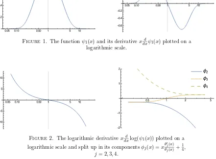
Figure 1. The function ψ1(x) and its derivative xd
dxψ1(x) plotted on a
logarithmic scale.
Figure 2. The logarithmic derivative xd
dxlog(ψ1(x)) plotted on a
logarithmic scale and split up in its components φj(x) =xθ′j(x) θj(x)+
References
[1] Albert Baernstein II. Landau’s constant, and extremal problems involving discrete subsets ofC. In Vik-tor P. Havin and Nikolai K. Nikolski, ediVik-tors, Linear and Complex Analyis Problem Book 3, Part 2, number 1574 in Lecture Notes in Mathematics, chapter 18, pages 404–407. Springer, 1994.
[2] Albert Baernstein II. A minimum problem for heat kernels of flat tori. InExtremal Riemann surfaces (San
Francisco, CA, 1995), volume 201 ofContemp. Math., pages 227–243. Amer. Math. Soc., Providence, RI,
1997.
[3] Albert Baernstein II and Jade P. Vinson. Local Minimality Results Related to the Bloch and Landau Constants. In Peter Duren, Juha Heinonen, Brad Osgood, and Bruce Palka, editors, Quasiconformal
Mappings and Analysis: A Collection of Papers Honoring F.W. Gehring, pages 55–89. Springer New
York, New York, NY, 1998.
[4] Laurent B´etermin and Mircea Petrache. Dimension reduction techniques for the minimization of theta functions on lattices.Journal of Mathematical Physics, 58(7):071902, 2017.
[5] Mark Coffey and George Csordas. On the log-concavity of a Jacobi theta function.Mathematics of
Com-putation, 82(284):2265–2272, 2013.
[6] Henry Cohn, Abhinav Kumar, Stephen D. Miller, Danylo Radchenko, and Maryna S. Viazovska. The sphere packing problem in dimension 24.Annals of Mathematics, 187(3):1035–1068, 2017.
[7] John H. Conway and Neil J. A. Sloane.Sphere packings, lattices and groups, volume 290 ofGrundlehren
der Mathematischen Wissenschaften [Fundamental Principles of Mathematical Sciences]. Springer-Verlag,
New York, third edition, 1998.
[8] George Csordas. Fourier Transforms of Positive Definite Kernels and the Riemannξ -Function.
Compu-tational Methods and Function Theory, 15(3):373–391, Sep 2015.
[9] Anne-Maria Ernvall-Hyt¨onen and Esa V. Vesalainen. On a conjecture of Faulhuber and Steinerberger on the logarithmic derivative ofϑ4.arXiv preprint arXiv:1709.05194, 2017.
[10] Markus Faulhuber.Extremal Bounds of Gaussian Gabor Frames and Properties of Jacobi’s Theta
Func-tions. PhD thesis, University of Vienna, 2016.
[11] Markus Faulhuber. Minimal Frame Operator Norms Via Minimal Theta Functions.Journal of Fourier
Analysis and Applications, pages 1–15, 2017.
[12] Markus Faulhuber and Stefan Steinerberger. Optimal Gabor frame bounds for separable lattices and estimates for Jacobi theta functions.Journal of Mathematical Analysis and Applications, 445(1):407–422, January 2017.
[13] Beverly Hernandez. Results on the Secrecy Function Conjecture on the Theta Function of Lattices. Mas-ter’s thesis, California State University, Northridge, 2016.
[14] Augustus J. E. M. Janssen. Some Weyl-Heisenberg frame bound calculations.Indagationes Mathematicae, 7(2):165–183, 1996.
[15] Hugh L. Montgomery. Minimal theta functions.Glasgow Mathematical Journal, 30:75–85, January 1988. [16] Elias Stein and Rami Shakarchi.Complex Analysis. Princeton University Press, Princeton, NJ, 2003. [17] Esa V. Vesalainen and Anne-Maria Ernvall-Hyt¨onen. Personal communication.
[18] Esa V. Vesalainen and Anne-Maria Ernvall-Hyt¨onen. On the secrecy gain of ℓ-modular lattices.arXiv
preprint arXiv:1708.09239, 2017.
[19] Maryna S. Viazovska. The sphere packing problem in dimension 8.Annals of Mathematics, 187(3):991– 1015, 2017.