TLS FIELD DATA BASED INTENSITY CORRECTION FOR FOREST ENVIRONMENTS
J. Heinzel* and M.O. Huber
WSL Swiss Federal Institute for Forest, Snow and Landscape Research, Zürcherstraße 111, 8903 Birmensdorf, Switzerland - (johannes.heinzel, markus.huber)@wsl.ch
Commission VIII, WG VIII/7
KEY WORDS: Terrestrial Laser Scanning, Forestry, Signal Amplitude, Intensity Correction
ABSTRACT:
Terrestrial laser scanning (TLS) is increasingly used for forestry applications. Besides the three dimensional point coordinates, the 'intensity' of the reflected signal plays an important role in forestry and vegetation studies. The benefit of the signal intensity is caused by the wavelength of the laser that is within the near infrared (NIR) for most scanners. The NIR is highly indicative for various vegetation characteristics.
However, the intensity as recorded by most terrestrial scanners is distorted by both external and scanner specific factors. Since details about system internal alteration of the signal are often unknown to the user, model driven approaches are impractical. On the other hand, existing data driven calibration procedures require laborious acquisition of separate reference datasets or areas of homogenous reflection characteristics from the field data.
In order to fill this gap, the present study introduces an approach to correct unwanted intensity variations directly from the point cloud of the field data. The focus is on the variation over range and sensor specific distortions. Instead of an absolute calibration of the values, a relative correction within the dataset is sufficient for most forestry applications. Finally, a method similar to time series detrending is presented with the only pre-condition of a relative equal distribution of forest objects and materials over range.
Our test data covers 50 terrestrial scans captured with a FARO Focus 3D S120 scanner using a laser wavelength of 905 nm. Practical tests demonstrate that our correction method removes range and scanner based alterations of the intensity.
1. INTRODUCTION
1.1 General overview
Terrestrial laser scanning (TLS) data is increasingly used as a ground based remote sensing data source. Similar to its airborne counterpart (airborne laser scanning – ALS) established fields of application for TLS data are forest and vegetation studies. In contrast to optical photographic data it allows to extract information from inside the vegetation structure with high precision. TLS is both used on its own and in combination with ALS data. While airborne data provides area wide coverage, terrestrial data is often used on a sample plot basis to provide local data with much higher resolution and from a ground based perspective.
The three dimensional point cloud is often regarded as the principle geometric information of light detection and ranging (LiDAR). In addition, radiometric information which can be derived from the strength of the reflected signal of the laser beam, is of special importance for vegetation studies. This is caused by the wavelength of the laser that is within the near infrared (NIR) for most scanners. The NIR is highly indicative for various vegetation characteristics and has been used in remote sensing for applications like tree species detection and tree damage assessment. However, the intensity as recorded by most terrestrial scanners is distorted by both external and scanner specific factors. While it varies over range and with incident angle onto the reflecting object, TLS systems themselves also cause alterations of the recorded intensity values. Details of the latter are mostly unknown to the user, which makes model driven correction approaches impractical. Several authors already addressed the problem of intensity correction of LiDAR data and some focused on the special problems of TLS. Höfle and Pfeifer (2007) concentrate on airborne data but generally compare model and data driven correction approaches. They demonstrate that even if both methods provide comparable results for ALS data, the model
driven approach requires detailed information on system settings and external conditions. Based on this, Pfeifer et al. (2007) and Pfeifer et al. (2008) investigate the correction of intensity data for TLS more specifically. Again, they compare model and data driven approaches. For TLS, they explain that model driven approaches are practically not working, mainly due to the lack of important scanner specific parameters, which are not disclosed by the manufacturer. Furthermore, they describe the scanner to object distance as a major factor for intensity variations. Since sole application of the inverse-square-law to this relationship is not sufficient for TLS data (Höfle, 2014; Pfeifer et al., 2007), they use measurements from reference targets recorded with a special calibration setup. This extensive procedure requires multiple targets of known and varying reflectivity and is separate from any field measurements.
Kaasalainen et al. (2011), Kaasalainen et al. (2009) and Kaasalainen et al. (2008) published a series of studies which also make use of reference targets in order to calibrate intensity. They observe the relationship between intensity and different interactive variables in detail. Their main focus is on the distance of scanner to object as well as the incident angle. Those are considered to be of major influence to the intensity besides the reflective properties of the object.
Höfle (2014), Koenig et al. (2015) and Koenig et al. (2013) use a less complex approach without calibrated reference targets which is based on the method used before by Höfle and Pfeifer (2007) for ALS data. From the TLS data, as recorded for an agricultural application, they extract large surface areas of homogenous soil to use them as reference for relative calibration of the remaining point cloud. This approach already comes close to the intention of the present study aiming at a practical application-oriented solution without any separate calibration setup. The disadvantage of their approach is that it requires environmental conditions that provide large continuous and homogenous areas, which are rarely available for forest applications. Additionally, the manual extraction of those areas
prevents automation of the method and increases the operational effort.
1.2 Intensity effects of TLS data
Variation of the intensity may have different sources. The term 'intensity' is somehow inaccurate in its physical meaning. In the context of this study, intensity is considered to be the amplitude of the reflected signal and both terms are used interchangeably. However, different manufacturers of scanners may measure and define the amplitude with certain deviations (Pfeifer et al., 2008).
Intensity variation can generally be caused either by characteristics of the reflecting object itself or by object-independent sources. Of primary interest is the isolation of the object-specific intensity variations by compensating the others. This allows conclusions about certain radiometric features of the objects. The group of other influences can be subdivided into scanner-specific and external sources. The effects of non-object-specific factors often differentiates strongly between TLS and ALS data. For example, the atmospheric influence is almost neglectable in case of TLS, while the distance between scanner and object has much stronger effects on TLS data. The latter is based on the fact that for TLS specific applications, the relative range differences between objects and scanner vary much stronger than for ALS. This results in range being one of the most relevant factors for explaining object-independent intensity variations (Höfle, 2014; Koenig et al., 2015; Koenig et al., 2013; Pfeifer et al., 2008). Also, range dependency of TLS in near distance applications does not strictly follow the 1/r2 law of the radar equation, as is the case for ALS (Höfle, 2014). This is mainly caused by a number of system-related alterations from the scanner and receiver device. Many of these system related alterations also depend on the range (Kaasalainen et al., 2008) and effect the function of intensity versus range. Therefore, data driven approaches to correct the range dependency of the intensity also compensate many of those alterations caused by the system receiver.
Depending on the manufacturer and model of the terrestrial scanner, different alterations of the received signal may be applied. This is expressed by the different shapes of the curves when plotting intensity against range for scanners from different manufacturers, e.g. RIEGL and Optech (Pfeifer et al., 2008), FARO (Kaasalainen et al., 2008) or devices from Leica (Kaasalainen et al., 2011; Kaasalainen et al., 2009). For the present study we use a FARO Focus 3D S120 scanner. In the studies of Kaasalainen et al. (2011), Kaasalainen et al. (2009) and Kaasalainen et al. (2008), a FARO scanner is used as well, but a different model. Since the shape of the intensity-range graphs are very similar to ours (see Figure 5), we assume that similar system-specific alterations are applied. The authors report the following alterations as conclusions from laboratory analysis. For small reflectances a logarithmic amplifier is used. This could result in partly compensated loss of amplitude for objects at larger distances. For near distances, a brightness reducer is used which results in a decrease of intensity at close distances. It is assumed that these modifications produce a specific pattern on the general amplitude-range distribution.
2. METHOD
2.1 Data
Data for this study has been collected in the field between spring and autumn 2015. The study area comprises the regions
Herrschaft andSchanfigg in the canton Grisons, Switzerland. Scans have been made on spatially separated plots of squared shape with an edge length of 25 m. Altogether, ten spatially
separated plots have been used in this study which are evenly split between both locations. On each plot, five terrestrial scans have been made, four being located towards the corners and one in the centre. Altogether it sums up to 50 scans being available. In order to register the single scans into a common coordinate system, six spheres have been fixed on ranging poles of varying length and distributed over the plot area. The spheres have a diameter of 145 mm and are of highly reflective white colour. Differentially corrected GNSS measurements from scanner and sphere positions were used for geocoding of the data.
The scanner model used is a FARO Focus 3D S120 which applies phase shift technology for range measurement. The wavelength of the laser is 905 nm and close to the lower border of the NIR. The emitted beam has a diameter of 3 mm with a divergence angle of 0.19 mrad. One of the experiments required the isolation of reflections from the spheres. This was done manually with specific tools from the FARO SCENE software. The same software was used for registration of the single scans, basic outlier filtering and clipping the data to a maximum range of 100 m from the scanner.
The wavelength of the laser at 905 nm seems to be non-optimal for the discrimination of vegetation characteristics and materials. Generally, LiDAR intensity has proven to be useful in the distinction of wood and leave components (Béland et al., 2011; Seielstad et al., 2011) and especially from ALS data for the classification of tree species (Heinzel and Koch, 2011; Heinzel and Koch, 2012; Kim et al., 2009). Most of these studies which applied LiDAR intensity successfully used scanners with a wavelength clearly above 1000 nm and mostly at about 1500 nm. Visualization of the uncorrected 905 nm data as recorded by the scanner system did not allow clear dinstinction of vegetation characteristics. The same observation has been confirmed by Pimont et al. (2015), where a detailed discussion of this phenomenon can be found. However, this motivated us to experiment with the automation of intensity correction methods directly from the field data.
2.2 Detrending the intensity distribution
The method for intensity correction described in this study is similar to the so called 'time series detrending'. Time series detrending is originally used to detect and compensate trends of a variable over time. In this study, we refer to the description of an intrinsic trend as defined by Wu et al. (2007), but we transfer this concept to a trend over range which exhibits similar behaviour.
The principal task for implementing the technique of detrending is to derive a model which describes the trend of the amplitude distribution. This model is used to correct the whole dataset for those amplitude variations referring to the overall trend while preserving those deriving from reflection characteristics of the objects. Experimentally, two different approaches to derive those models have been tested.
The first approach fits a polynomial to the amplitude data of the complete point cloud. The polynomial is directly used to correct the amplitude values by division with the corresponding polynomial values at same distance from the scanner. In order to optimize the degree of the polynomial, we implemented an-fold cross validation iterating over the central scans of spatially independentn plots. With each step, the degree of the polynomial is increased by one and the polynomial is fitted by the least-squares method to the merged points from nine out of ten plots. The left out plot is iteratively used to test the derived polynomial and the residuals are calculated. For each polynomial degree, these residuals are summed for all iterations. The minimum value of this series is determined and represents the optimal degree of the polynomial. In order to reduce the influence of outliers, we apply weights to all points prior to the iterative procedure. Outliers are defined as those points deviating more than two times the standard deviation within a range bin of 1 m. Figure 1 shows the complete procedure of polynomial optimization.
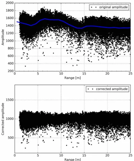
The second approach to model the overall trend substitutes the polynomial by calculating the mean values of the amplitude at small range intervals. The whole dataset is binned into constant range intervals of defined size. For each bin, the mean amplitude is computed. Finally, all amplitudes within one bin are divided by their corresponding mean. In order to scale the corrected amplitudes to a data range allowing 16 bit unsigned integer encoding and which makes them comparable to the original values, they are multiplied by the factor 1000.
3. EXPERIMENTS
3.1 Field data based correction
The first experiment directly handles the complete point cloud as captured in the field. This means that all points independent from their source of reflection are used to derive the model for correction. Both the polynomial optimization as well as the binned mean approach are tested with that data. Results are presented for a single isolated scan.
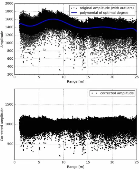
For the polynomial approach, the degree of the polynomial was optimized using the central scans of all plots in a 10-fold cross-validation procedure. The optimization results in a polynomial of twelfth degree. The upper part of Figure 2 shows the original amplitudes plotted against range. The blue line represents the polynomial of optimal degree and the non filled dots indicate outliers. The lower graph of the figure displays the corrected amplitude centred at a value of 1000.
The second approach calculates the mean amplitude values for bin sizes of 1 m on the range axis. Figure 3 shows the corresponding scatterplots for the same scan as in Figure 2. In the upper graph of the figure, the blue line indicates the mean amplitude values for the original point cloud. The lower graph Figure 2. Amplitude correction by fitting a polynomial. Top: The original amplitude plotted against range. The lighter non filled dots indicate outliers. Bottom: the corrected amplitude centred at a value of 1000.
displays the distribution of the corrected amplitude values versus range.
3.2 Sphere based correction
In addition to the direct correction of the complete point data at once, a second experiment was carried out. This experiment takes on the role of a relative reference to be compared to the outcome of the field data based correction. Isolated reflections from the spheres were used as substitutes for special calibration targets. In this context, we take advantage of the equal reflection characteristics. Compensation for varying incident angles was achieved by calculating the arithmetic means for all amplitudes from each sphere. This was done for the spheres in all 50 scans and resulted in 232 averaged samples. The experiment produces results which are principally comparable to other approaches using special calibration targets to derive absolute (Höfle and Pfeifer, 2007; Pfeifer et al., 2008) or relative (Höfle, 2014; Kaasalainen et al., 2008) calibration models.
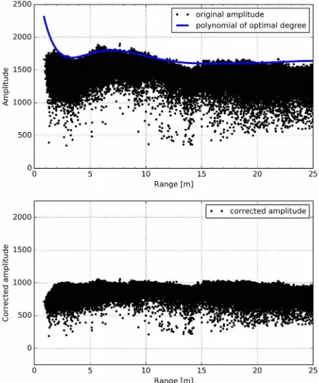
The reference reflections from the spheres underwent the same processing steps as the complete point cloud of the previous experiment. Firstly, the optimal degree and the coefficients of the polynomial fitted to the spheres samples were determined. Figure 4 illustrates the finding of the optimal polynomial of eighth degree for a 10-fold cross validation. The degree of the polynomial is smaller since the maximum range of spheres reflection is only 25 m. Figure 5 applies the optimized polynomial to the sphere samples. The upper graph shows the distribution of the averaged amplitudes with the polynomial modelling the overall trend. The lower graph plots the corresponding corrected spheres amplitudes.
For reference and comparison, some quality metrics have been computed for this experiment. Fitting the optimal polynomial to the spheres produces a root mean square error (RMSE) of 29.37 on the original scale. The same RMSE for intensities being normalized to their maximum value equals 0.0156. Furthermore, the normalized RMSE (NRMSE) was derived according to equation (1) which is equal to 0.0836.
NRMSE
=
√
∑
i=1n
( ^
y
i−
y
i)
2
y
max−
y
min(1)
In equation (1)n is the number of data points (spheres),ŷi is the predicted amplitude forith sample of amplitudey,ymax is the
maximum and ymin is the minimum amplitude of the dataset. To be complete, the polynomial derived from the spheres is also applied to the full set of field data. Figure 6 shows the results for this combination in the same form as the previous figures.
4. RESULTS AND DISCUSSION
The results of the first experiment are provided in form of graphs in Figure 2 a n d Figure 3. The first approach for modelling amplitude data fits an optimized polynomial to all reflections from the data set. The upper graph of Figure 2 shows the polynomial modelling the overall trend for all reflections from one scan. While the polynomial was fitted to the complete range of distances of 100 m from the scanner, the figure only displays the first 25 m, where the strongest variations are located. From the lower graph it can be seen that the intrinsic trend and large scale variations are largely removed while the local variations around the polynomial are preserved.
The same graphs are given for the binned means approach in Figure 3. The curve of mean values is less smooth and reflects local variations of the amplitude distribution more precisely than the polynomial. While this might be an advantage in cases where the polynomial generalizes too much, it might also happen that the binned means result in an overfitting to the data. The distribution of the corrected amplitude in the lower part of the figure reveals a very smooth upper boundary. This is caused by the locally adapted fit of the mean values to the dataset and possibly indicates the tendency for overfitting. In this context, overfitting largely depends on the size of the bin intervals. Figure 4. Mean residuals of the test data from a 10-fold cross-validation. The cross validation has been carried out for a series of polynomial degrees. The degree with the minimum residuals has been selected.
The coefficients of variation (CV) in the upper part of Table 1 lead to similar observations. The table compares the CVs for the first experiment over the complete data range. From there it can be seen that the corrected amplitude has a slightly lower CV for the binned means compared to the polynomial variant. This is proportionate to the smoother upper boundary of the scatterplots. However, the differences are only small and hardly effect any practical interpretation of the amplitude.
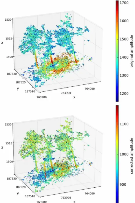
Figure 7 provides a three-dimensional visualization of the point cloud with colour coded amplitudes. The upper graph shows the original amplitudes and the lower part the polynomially corrected amplitudes. The figure omits a separate graph with amplitudes corrected by binned mean values because no difference to the polynomial correction could be found visually. For the original amplitudes, it can be clearly seen that the highest amplitudes accumulate at around seven meters distance. This refers to the maximum of the polynomial at the same distance in Figures 2 and 3. For the polynomially corrected graph, the range dependent amplitude variations are largely eliminated. This demonstrates the practical effectiveness of the correction method.
The second experiment serves as a reference to be compared to the direct field data based approach. Only the isolated reflections from the homogenously reflecting spheres are used to fit a polynomial. Figure 5 illustrates the resulting curve as well as the distribution of the original and the corrected amplitudes. It can be clearly seen that the shape of the curve and the location of the maxima and minima match the curves derived from the complete dataset (compare Figures 2 and 3). This is an indication for the quality of the direct field data based correction. Moreover, the limitation to equal reflectors results in a much smaller local variance of the amplitudes below and above the curve. It allows a more distinct fit of the polynomial. The remaining local variation can be explained in large part by mixing spheres from different plots and being scanned at different times and places. In this context, Kaasalainen et al. (2008) and Kaasalainen et al. (2010) point to the influence of varying background noise, temperature and moisture. Another disturbing factor might be the strongly unequal number of reflections on the spheres depending on their distance from the scanner.
I n Figure 6, the polynomial derived from isolated spheres is applied to the complete field data. The distribution of the corrected field data in the lower graph is comparable to the corrected field data from the first experiment. Due to the higher mean amplitudes of the spheres, the polynomial results in a shift on the y-axis while the general shape is preserved. This indicates again that fitting the polynomial directly to the complete point cloud provides sound results and at the same time simplifies the workflow.
The statistical metrics of RMSE and NRMSE as provided in section 3.2 are relatively low and refer to a good fit of the polynomial to the amplitudes from the spheres. Höfle (2014) is one of the few authors providing quality metrics and experimental settings similar to our experiments. The main difference is that he uses homogenous ground areas from an agricultural application as relative references. While the course of the overall trend of his dataset differs strongly from the present data, the reported optimal degree of the polynomial is the same. The RMSE for all reflections in his study is 0.0229 whereas the present study achieves a significantly smaller error of only 0.0156. Both RMSEs are made comparable by normalizing the dataset with the maximum value. The numbers reveal that the reference source of highly reflective spheres could be superior to the extraction of homogenous areas of the Figure 5. Top: Distribution of the original amplitude over range
for all spheres on all plots. The reflections of each sphere have been averaged. The line visualizes the polynomial of optimal degree fitted to the distribution of amplitudes. Bottom: The distribution of amplitudes after polynomial correction.
environment. Another practical advantage of the spheres is that they are used by default for any scan campaign, while large homogenous areas do not exist in sufficient quantity in complex environments such as forests.
The lower part of Table 1 lists the CVs for the spheres derived amplitudes and the complete point cloud corrected by the spheres polynomial. Since the maximum available distance for spheres is 25 m, the CVs of the first experiment are recomputed for this reduced distance. The values in the table reflect the low variation of the isolated spheres amplitudes. Surprisingly, when applying the spheres polynomial to the complete dataset, the difference in variation between corrected and uncorrected amplitudes remains very small. Compared to the first experiment this might be explained by stronger generalization due to much less spheres reflections being available for polynomial fitting. Though, a visualization of the colour coded amplitudes corrected by the spheres polynomial does not noticeably differ from the direct field data correction in the lower graph of Figure 7.
Experimental setting
C o e f f i c i e n t o f variation (original amplitude)
C o e f f i c i e n t o f variation (corrected amplitude)
Full range of 100m
Polynomial from complete point cloud
0.0926 0.0825
Binned means of complete point cloud
0.0926 0.0813
Reduced range of 25 m
Polynomial from complete point cloud
0.0963 0.0837
Binned means of complete point cloud
0.0963 0.0831
Polynomial from isolated sphere reflections
0.0476 0.0174
Spheres derived p o l y n o m i a l t o complete point cloud
0.0963 0.0936
Table 1. Comparison of the coefficients of variation before and after correction of the amplitudes. The coefficients are listed for different experimental settings. The upper part of the table shows values for the full data range of 100 m and the lower part is limited to 25 m, which is the maximum distance of the spheres.
Generally, all presented indications confirm the quality of the direct correction of the complete field data as described in the first experiment. Results show no visible inaccuracies in comparison to the reference from isolated spheres. The direct method achieves full automation and does not require any calibration targets. From the two approaches being tested, the polynomial approach is preferred since it provides stable results on all of our scans while not being prone to overfitting. Since the curve of the trend exhibits the same typical pattern over all scans and plots, we assume that it is specific for this model of
scanner. This justifies the option to apply the optimized polynomial to all scans from all plots and reinforces the application oriented character of the methodology. The only preassumption for the described method is a homogenous distribution of objects and materials over range for each scan. This assumption is required to minimize the effects of object induced local variances on the global trend. For scan settings in most forest stands, the pre-condition should be fulfilled sufficiently. Materials and objects such as wood, soil, green leaves and needles occur equally at all distances from the scanner. For practical application, a roughly equal distribution should be sufficient. Furthermore, the range dependent distribution disregards the direction in which objects occur.
5. CONCLUSIONS
extraction of homogenous reference structures from the scan environment are required. This guarantees independency and a high degree of automation. The only pre-condition for the described methodology is a relatively homogenous distribution of objects and materials over range. For most forestry applications, this is fulfilled to a sufficient degree.
The presented results suggest that fitting a polynomial of optimal degree directly to the complete point cloud should be the preferred variant of the methods described. This avoids overfitting in comparison to the binned means variant and requires less effort than extracting points from registration spheres on the plot. Also, the graphical plots, the coefficients of variation and the visualization of colour coded amplitudes support this conclusion.
For future research, a comparison with absolute calibration targets would be interesting. This could reinforce our observations with more quantitative evidence.
ACKNOWLEDGEMENTS
The authors would like to thank Natalia Rehush and Björn Dreier for their strong support in field work as well as Christian Ginzler for his expertise in GNSS technology and registration of the scans. Special thanks also go to the forest administration of the canton Grisons, Switzerland, who gave important assistance to this project.
REFERENCES
Béland, M., Widlowski, J.-L., Fournier, R. A., Côté, J.-F. and Verstraete, M. M., 2011. Estimating leaf area distribution in savanna trees from terrestrial LiDAR measurements.
Agricultural and Forest Meteorology, 151(9), pp. 1252-1266.
Heinzel, J. and Koch, B., 2011. Exploring full-waveform LiDAR parameters for tree species classification.International Journal of Applied Earth Observation and Geoinformation, 13(1), pp. 152-160.
Heinzel, J. and Koch, B., 2012. Investigating multiple data sources for tree species classification in temperate forest and use for single tree delineation.International Journal of Applied Earth Observation and Geoinformation, 18, pp. 101-110.
Höfle, B., 2014. Radiometric correction of terrestrial LiDAR point cloud data for individual maize plant detection.
Geoscience and Remote Sensing Letters, IEEE, 11(1), pp. 94-98.
Höfle, B. and Pfeifer, N., 2007. Correction of laser scanning intensity data: Data and model-driven approaches.ISPRS Journal of Photogrammetry and Remote Sensing, 62(6), pp. 415-433.
Kaasalainen, S., Jaakkola, A., Kaasalainen, M., Krooks, A. and Kukko, A., 2011. Analysis of incidence angle and distance effects on terrestrial laser scanner intensity: Search for correction methods. Remote Sensing, 3(10), pp. 2207-2221.
Kaasalainen, S., Krooks, A., Kukko, A. and Kaartinen, H., 2009. Radiometric calibration of terrestrial laser scanners with external reference targets. Remote Sensing, 1(3), pp. 144-158.
Kaasalainen, S., Kukko, A., Lindroos, T., Litkey, P., Kaartinen, H., Hyyppa, J. and Ahokas, E., 2008. Brightness Measurements and Calibration With Airborne and Terrestrial Laser Scanners.
IEEE Transactions on Geoscience and Remote Sensing, 46(2), pp. 528-534.
Kaasalainen, S., Niittymaki, H., Krooks, A., Koch, K., Kaartinen, H., Vain, A. and Hyyppa, H., 2010. Effect of Target Moisture on Laser Scanner Intensity.IEEE Transactions on Geoscience and Remote Sensing, 48(4), pp. 2128-2136.
Kim, S., McGaughey, R. J., Andersen, H.-E. and Schreuder, G., 2009. Tree species differentiation using intensity data derived from leaf-on and leaf-off airborne laser scanner data.Remote Sensing of Environment, 113(8), pp. 1575-1586.
Koenig, K., Höfle, B., Hämmerle, M., Jarmer, T., Siegmann, B. and Lilienthal, H., 2015. Comparative classification analysis of post-harvest growth detection from terrestrial LiDAR point c l o u d s i n p r e c i s i o n a g r i c u l t u r e .ISPRS Journal of Photogrammetry and Remote Sensing, 104, pp. 112-125.
Koenig, K., Höfle, B., Müller, L., Hämmerle, M., Jarmer, T., Siegmann, B. and Lilienthal, H., 2013. Radiometric correction of terrestrial lidar data for mapping of harvest residues density. In:Annals of the Photogrammetry, Remote Sensing and Spatial Information Sciences, Vol. 2, pp. 133-138.
Pfeifer, N., Dorninger, P., Haring, A. and Fan, H., 2007. Investigating terrestrial laser scanning intensity data: quality and functional relations. In:Proceedings of the 8th Conference on Optical 3-D Measurement Techniques, Zurich, Switzerland, pp. 328–337.
Pfeifer, N., Höfle, B., Briese, C., Rutzinger, M. and Haring, A., 2008. Analysis of the backscattered energy in terrestrial laser scanning data. In:The International Archives of the Photogrammetry, Remote Sensing and Spatial Information Sciences, Beijing, China, Vol. XXXVII Part B5, pp. 1045-1052.
Pimont, F., Dupuy, J.-L., Rigolot, E., Prat, V. and Piboule, A., 2015. Estimating Leaf Bulk Density Distribution in a Tree Canopy Using Terrestrial LiDAR and a Straightforward Calibration Procedure. Remote Sensing, 7(6), pp. 7995-8018.
Seielstad, C., Stonesifer, C., Rowell, E. and Queen, L., 2011. Deriving fuel mass by size class in Douglas-fir (Pseudotsuga menziesii) using terrestrial laser scanning.Remote Sensing, 3(8), pp. 1691-1709.