ESTIMATION OF TREE STEM ATTRIBUTES USING TERRESTRIAL
PHOTOGRAMMETRY
Mona Forsmana,∗and Niclas B¨orlinband Johan Holmgrena a
Department of Forest Resource Management, Section of Remote Sensing, Swedish University of Agricultural Sciences, Ume˚a, Sweden - (mona.forsman,johan.holmgren)@slu.se, http://www.slu.se/srh
b
Department of Computing Science, Ume˚a University, Ume˚a, Sweden - [email protected]
Commission V/4
KEY WORDS:Measurement, Image, Algorithms, Forestry, Inventory, Point Cloud, Close Range, Method
ABSTRACT:
The objective of this work was to create a method to measure stem attributes of standing trees on field plots in the forest using terrestrial photogrammetry. The primary attributes of interest are the position and the diameter at breast height (DBH).
The developed method creates point clouds from images from three or more calibrated cameras attached to a calibrated rig. SIFT features in multiple images in combination with epipolar line filtering are used to make high quality matching in images with large amounts of similar features and many occlusions. After projection of the point cloud to a simulated ground plane, RANSAC filtering is applied, followed by circle fitting to the remaining points.
To evaluate the algorithm, a camera rig of five Canon digital system cameras with a baseline of 123 cm and up to 40 cm offset in height was constructed. The rig was used in a field campaign at the Remningstorp forest test area in southern Sweden. Ground truth was collected manually by surveying and manual measurements.
Initial results show estimated tree stem diameters within 10% of the ground truth. This suggest that terrestrial photogrammetry is a viable method to measure tree stem diameters on circular field plots.
1 INTRODUCTION
1.1 Background and Aim
The forestry industry requires information, such as species, stem diameter, volume and height, about trees in the forests for man-agement planning. Traditionally, the information has been col-lected by manual inventory using calipers to measure stem diam-eters. The inventory in Sweden is usually done on circular field plots with a radius of 10 meters. From this kind of samples larger stocks of forests are estimated. The process of manually measur-ing the trees is labor intensive, and the planners want as much and as reliable information as possible.
In this paper, a method to estimate tree stem diameter and position using terrestrial photogrammetry and image analysis is proposed.
1.2 Related work
There are only a few studies to be found on estimation of stem attributes using terrestrial stereophotogrammetry. The work by Reidelst¨urz (1997) was performed on analog images and con-cludes that manual measurements in analog images would be un-feasible due to long processing times. More recently, Hapca et al. (2007, 2008) present methods for stem profiling and measure-ment based on digital photogrammetry. However, this method places several constraints on the imaging process. The cameras must be accurately leveled and the images must be taken from two angles, separated by exactly 90◦. Furthermore, the scene must be
modified to include a marking of a known distance. The paper by Abd-Elrahman et al. (2010) presents a method for inventory of trees in urban areas using images taken by the general public. The presented method is based on manual measurements in dig-ital images and is evaluated on free-standing trees in a number of parks. The analysis time for a set of 6–12 images is cited as
∗Corresponding author
4–8 hours. The report by Larsson et al. (2011) studies the related problem of sensor technology to be mounted on harvesters to col-lect forestry data during harvesting. The sensors include a pair of video cameras, a 2D line scanner (SICK LMS-511), and a short range flash sensor (PMDTec Camcube).
2 MATERIALS AND METHOD
2.1 Camera rig
2.1.1 Hardware A camera rig consisting of five digital sys-tem cameras with a total baseline of 123 cm and up to 40 cm off-set in height was built (Figure 1). Three Canon EOS 7D equipped with Sigma EX20/1.8 DG wide angle lenses and two Canon EOS 40D equipped with Canon EF-s 17–55/2.8 zoom lenses, locked at 17 mm, were mounted to the rig. The cameras were synchro-nized by a cable trigger to ensure the images were taken at the same time. A magnetic field compass was attached to the rig to make it easier to evenly distribute the exposures in a circle.
Five cameras were used for two reasons. Firstly, offset-mounted additional cameras reduce the risk of false matches due to am-biguities in epipolar matching between only two cameras. Sec-ondly, the larger number of cameras reduces the risk of occlusion problems, in an environment where branches and leaves at short range from the cameras are common.
The total weight of the rig was about 13.5 kg. The rig can be used with a common camera tripod. However, this would be cumber-some to carry around and adjust in the terrain. Instead, Easyrig 2.51, a portable camera support system originally developed for
TV cameras, was preferred (Figure 1).
1www.easyrig.com
Figure 1: The five-camera rig in the field, carried with Easyrig 2.5.
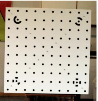
Figure 2: The PhotoModeler camera calibration sheet printed on a sheet of aluminium. Stringers were attached to the back of the sheet for additional stability.
2.1.2 Calibration To investigate the stability of the camera and lens before they were mounted on the rig, each of the eras was calibrated multiple times using the PhotoModeler cam-era calibration sheet2 and in-house camera calibration software
(B¨orlin et al., 2004). For additional stability, the calibration sheet (Figure 2) was printed on an aluminium sheet with attached string-ers. Over 20 calibration images were used for each camera cali-bration to cover different camera rotations, camera-to-object dis-tances, and all of the CCD. The cameras were calibrated four to ten times each during a period of two months. The variation in focal length estimation during this period was below 0.03 mm.
The camera rig was calibrated by bundle adjustment of one expo-sure of the same calibration sheet. The calibration was repeated on a regular basis during the campaign to reduce any handling effects.
2.2 Field work
2.2.1 Data acquisition protocol Within each circular field plot, images were acquired from five positions. At every position, ex-posures were taken in each of 12 directions separated by approx-imately 30 degrees as shown in Figure 3. Two sets of images were taken in each direction to increase redundancy and to guard against problems with the exposure. The camera rig was cali-brated before and after every plot using the procedure described
2www.photomodeler.com
Figure 3: The image acquisition protocol for each field plot con-sisted of a central camera station and four satellite stations. The satellite stations were approximately 10 m from the center in the four cardinal directions. At each station, images were taken in 12 directions separated by approximately 30 degrees.
in Section 2.1.2. Each exposure was furthermore recorded in a written protocol.
2.2.2 Campaign In August 2011, a field campaign was un-dertaken to the Remningstorp test area outside Sk¨ovde in south-ern Sweden (N58.46◦, E013.65◦). The forest at Remningstorp is
semi-boreal with mostly Scotch Pine, Norway Spruce and some broad-leaved trees.
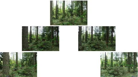
During three days of field work, 25 field plots with 20 m radius were photographed using the five-camera rig. An example of a single five camera exposure is shown in Figure 4. The weather during the campaign was mostly sunny with scattered clouds, with some period of broken clouds and light rain. In total, about 25 000 images summing up to 175 GB of data was collected.
Approximately 20–30 minutes were spent on each plot. This time covers image acquisition including rig pre- and post-calibration, transportation to and from the closest road as well as loading and unloading of the equipment from the car.
2.2.3 Ground truth For validation, the stem diameters at breast height (DBH) of all trees in the plots were manually measured separately using a caliper. Furthermore, tree positions within each plot were determined by a land surveyor using a total sta-tion. Additionally, the plots were laser scanned from the plot center with a Leica ScanStation C10.
3 ALGORITHMS AND ANALYSIS
3.1 Algorithms
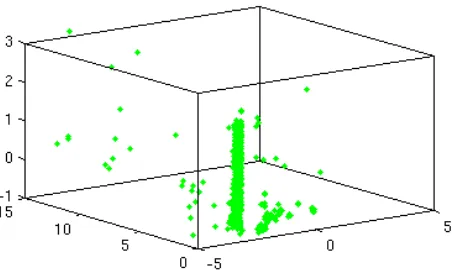
From each five-tuple of images acquired by the rig, a point cloud is constructed from feature points detected by SIFT (Lowe, 2004). Epipolar constraints (Hartley and Zisserman, 2003) are used to minimize false matches. Figure 4 shows a set of images from the camera rig. In the generated point clouds, some vertical clusters representing tree stems are obvious (Figure 5).
The points are projected on a ground plane, simulated by thex−z
plane in the rig coordinate system. A rough estimation of the stem diameter at breast height is acquired by circle fitting using RANSAC (Fischler and Bolles, 1981), the algebraic fit method by Gander et al. (1994) and a geometric fit method using Gauss-Newton (Gander et al., 1994; Nocedal and Wright, 2006).
3.1.1 Point cloud generation algorithm usingNcameras from a single viewpoint Given detected SIFT features in each image, a point cloud is generated by the following algorithm:
1. For each feature pointiin the reference camerar(typically the center camera)
1.1 Create a set of selected pointsS, initially containing the single pointifrom camerar.
1.2 For each other cameraj6=r
1.2.1 Create a set of candidate matchesCj, initially containing all feature points in imagej.
1.3 Select imageras the active image.
1.4 Repeat while there is at least one non-empty setCjof candidate matches
1.4.1 For each non-empty setCj
1.4.1.1 Filter the candidate matchesCj by the se-lected pointpin the active image. A candi-date pointq∈ Cjis removed if
• the descriptors ofqandpare too dissimi-lar, or
• the distance fromqto the epipolar line of
pis too large, or
• the qand pframe sizes differ too much, after compensation for the expected differ-ence due to potentially differing image res-olutions.
1.4.2 If there exists a setCjconsisting of a single point
k, the matching in imagejis unique:
1.4.2.1 Add the pointkin imagejto the setS of selected points.
1.4.2.2 Clear the setCjas the single remaining can-didate has been selected.
Figure 5: Part of a 3D point cloud. The trunk of a tree is clearly seen. The axis unit is meters.
1.4.2.3 Select imagejas the active image. 1.4.3 otherwise if there are non-empty sets left, the
matching is ambiguous in the remaining image(s): 1.4.3.1 Abandon the remaining images by clearing
the remaining non-empty setsCj.
1.5 If points were selected in at least three images, calcu-late a 3D point by forward intersection (McGlone et al., 2004).
An example of a generated 3D point cloud is shown in Figure 5.
3.1.2 Tree stem diameter measurements Given the 3D point cloud, tree diameters are calculated by the following algorithm:
1. Project the 3D point cloud to thex−zground plane (Fig-ure 6).
2. Segment the point cloud to find groups of points correspond-ing to a scorrespond-ingle tree. This is currently done manually.
3. Fit a circle to each segmented point cloud using RANSAC.
4. Fine-tune the circle to the remaining point using a Gauss-Newton algorithm.
3.2 Data selection
The images acquired from the central camera station of one field plot have been analyzed. The chosen plot is typical in the sense of having a variation in tree size and includes parts with only low undergrowth and other parts with brushwood. Spruce, pine, birch and other leaves are represented. As an initial data set, a total of twelve trees were chosen as the most clearly visible trees in the 3D point clouds.
4 PRELIMINARY RESULTS
An initial implementation of the algorithm of Section 3.1 has been applied to images from the center camera station from one of the field plots. Figure 4 shows an image set with matched fea-ture points marked. The green lines are epipolar lines for one of the points. The generated point clouds are sparse due to high values of the filtering thresholds in Step 1.4.1.1 of the algorithm, but enough points exist to make some trees easy to detect, see Figure 5.
In Figure 6, the points in Figure 5 have been projected to the
x−z plane and a subset of the points corresponding to a stem
Figure 4: A set of images from the five-camera rig. The relative positioning of the images indicate the relative position of the camera within the rig. The green lines are the epipolar lines for one point.
Figure 6: The point cloud of Figure 5 projected on thex−z
plane. The points in the red rectangle correspond to points on the tree trunk. The axis unit is meters.
has been manually indicated. In Figure 7, the indicated points have been filtered by RANSAC and circles have been fitted to the filtered points using three methods: The direct algebraic method by Gander et al. (1994) and two geometric fit methods using the Gauss-Newton algorithm (Gander et al., 1994; Nocedal and Wright, 2006). The unweighted geometric fit methods assumed isotropic point errors whereas the weighted geometric fit method assumed anisotropic point errors calculated by forward intersec-tion.
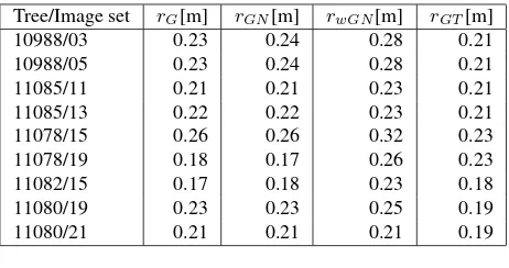
A set of stem radii, estimated by the above algorithms, are pre-sented in Table 1. All stems were positioned at a maximum dis-tance of approximately seven meters from the rig. Ground truth from caliper measurement is also displayed.
Figure 7: Three circles fitted by different methods to the points selected in Figure 6 after RANSAC filtering. Each point is indi-cated by its 1-sigma uncertainty ellipse. Some remaining outliers are seen, e.g. inside the circles near (-1.05,4.9) or outside the cir-cles near (-0.75,4.85). The blue circle is fitted using the direct al-gebraic method. The green circle was fitted by the Gauss-Newton algorithm assuming isotropic error.The red circle was fitted by the same algorithm assuming the errors indicated by the blue ellipses. The axis unit is meters.
Table 1: Estimated radii with the Gander method (rG), unweighted Gauss-Newton (rGN), weighted Gauss-Newton (rwGN) and measured ground truth (rGT).
Tree/Image set rG[m] rGN[m] rwGN[m] rGT[m]
10988/03 0.23 0.24 0.28 0.21
10988/05 0.23 0.24 0.28 0.21
11085/11 0.21 0.21 0.23 0.21
11085/13 0.22 0.22 0.23 0.21
11078/15 0.26 0.26 0.32 0.23
11078/19 0.18 0.17 0.26 0.23
11082/15 0.17 0.18 0.23 0.18
11080/19 0.23 0.23 0.25 0.19
11080/21 0.21 0.21 0.21 0.19
5 CONCLUSIONS AND FUTURE WORK
These preliminary results indicate that this method is viable for estimation of stem attributes in circular field plots. The method will be further developed and validated.
The current method appears to be sensitive to outliers remaining after the RANSAC filtering. This could be handled by levelling of the rig to obtain a better approximation of the ground plane followed by automatic exclusion of points too close to the ground. Circle fitting at different levels and/or fitting of a conical cylinder to the 3D point cloud could be used to handle the tapering of the stem. Furthermore, the RANSAC algorithm will be extended to handle anisotropic point errors. Additionally, the rig calibration will be improved to include multiple calibration images acquired at different distances to the calibration object.
One shortcoming in the current code is that small stems are hard to measure due to too few detected features. A possible improve-ment would be to co-register the point clouds from multiple expo-sures and camera positions in a field plot. The co-registration of the point clouds should also make it possible to create a tree map over the test site, which could be useful for different applications. Furthermore, comparisons of the stem diameter estimates will be performed with point clouds produced by a terrestrial laser scan-ner placed at the plot center.
ACKNOWLEDGEMENTS
This research was financed by the Kempe Foundations and by Hildur and Sven Wingquist Foundation for Forest Research.
References
Abd-Elrahman, A. H., Thornhill, M. E., Andreu, M. G. and Es-cobedo, F., 2010. A community-based urban forest inventory using online mapping services and consumer-grade digital im-ages. Int J Appl Earth Obs Geoinf 12(4), pp. 249–260.
B¨orlin, N., Grussenmeyer, P., Eriksson, J. and Lindstr¨om, P., 2004. Pros and cons of constrained and unconstrained formula-tion of the bundle adjustment problem. Internaformula-tional Archives of Photogrammetry, Remote Sensing, and Spatial Information Sciences XXXV(B3), pp. 589–594.
Fischler, M. A. and Bolles, R. C., 1981. Random sample con-sensus: A paradigm for model fitting with applications to im-age analysis and automated cartography. Comm ACM 24(6), pp. 381–395.
Gander, W., Golub, G. H. and Strebel, R., 1994. Least squares fitting of circles and ellipses. BIT 34, pp. 558–578.
Hapca, A., Mothe, F. and Leban, J.-M., 2007. A digital photo-graphic method for 3d reconstruction of standing tree shape. Annals of Forest Science (6), pp. 631–637.
Hapca, A., Mothe, F. and Leban, J.-M., 2008. Three-dimensional profile classification of standing trees using a stereopho-togrammetric method. Scand J Forest Res (23), pp. 46–52.
Hartley, R. I. and Zisserman, A., 2003. Multiple View Geometry in Computer Vision. 2nd edn, Cambridge University Press, ISBN: 0521540518.
Larsson, H., Engstr¨om, P. and Rydell, J., 2011. Measurement of tree population with new sensor technology at forest harvester. Technical Report FOI-D0443–SE, FOI, Swedish Defence Re-search Agency, Information Systems, Box 1165, SE-581 11 Link¨oping, Sweden.
Lowe, D. G., 2004. Distinctive image features from scale-invariant keypoints. Int J Comp Vis 60(2), pp. 91–110.
McGlone, C., Mikhail, E. and Bethel, J. (eds), 2004. Manual of Photogrammetry. 5th edn, ASPRS.
Nocedal, J. and Wright, S. J., 2006. Numerical Optimization. 2 edn, Springer-Verlag.
Reidelst¨urz, P., 1997. Forstliches Anwendungspotential der ter-restrisch - analytischen Stereophotogrammetrie. PhD thesis, der Albert-Ludwigs-Universit¨at Freiburg, Breisgau.