EVALUATION OF STEREO ALGORITHMS FOR OBSTACLE DETECTION WITH
FISHEYE LENSES
Nicola Krombach, David Droeschel, and Sven Behnke
Autonomous Intelligent Systems Group Institute for Computer Science VI
University of Bonn, Germany
(krombach,behnke)@cs.uni-bonn.de, [email protected]
KEY WORDS:MAVs, Stereo Cameras, Fisheye, Obstacle Detection
ABSTRACT:
For autonomous navigation of micro aerial vehicles (MAVs), a robust detection of obstacles with onboard sensors is necessary in order to avoid collisions. Cameras have the potential to perceive the surroundings of MAVs for the reconstruction of their 3D structure. We equipped our MAV with two fisheye stereo camera pairs to achieve an omnidirectional field-of-view. Most stereo algorithms are designed for the standard pinhole camera model, though. Hence, the distortion effects of the fisheye lenses must be properly modeled and model parameters must be identified by suitable calibration procedures. In this work, we evaluate the use of real-time stereo algorithms for depth reconstruction from fisheye cameras together with different methods for calibration. In our experiments, we focus on obstacles occurring in urban environments that are hard to detect due to their low diameter or homogeneous texture.
1. INTRODUCTION
In recent years, micro aerial vehicles (MAVs) such as multicopters have become increasingly popular as a research tool and for ap-plications like inspection tasks. Due to their low costs, small size, and the ability to hover, it is possible to reach locations, which are inaccessible or dangerous for humans or ground vehicles. Up to now, most MAVs are remotely controlled by a human operator and when constructing autonomous MAVs, payload limitations are one of the main challenges. Due to their small size and low weight, cameras are potential sensors for several tasks: from visual odometry over simultaneous localization and mapping (SLAM) and 3D surface reconstruction to visual obstacle detection. In contrast to infrared-based depth cameras, stereo vision works both indoors and outdoors, and does not suffer from scale ambiguity like monocular cameras do. Nevertheless, for computing accurate disparity maps they might require elaborate and slow stereo vi-sion processing. While for many uses, some errors in detection of visual features are acceptable, reliable navigation in complex 3D environments cannot tolerate missing detections, as the MAV could collide with them, nor false positive detections, as they restrict the free space the MAV needs for navigation.
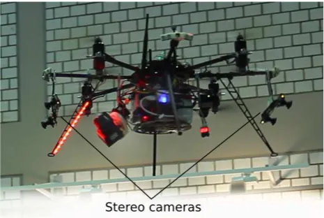
Our MAV, shown in Fig. 1, is equipped with four uEye 1221LE-M cameras forming two stereo camera pairs, facing forward and backward. For an omnidirectional view, the cameras are equipped with fisheye lenses—each with a field of view of up to180◦. To ensure reliable obstacle detection, a continuously rotating 3D laser scanner (Droeschel et al., 2014) and a ring of ultrasound sensors are used. The cameras provide dense measurements with high frequency in comparison to the other sensors: They capture images with20 Hzwhile the laser scanner operates with2 Hz. We use the MAV for autonomous navigation in the vicinity of obstacles (Droeschel et al., 2015).
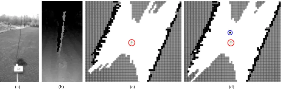
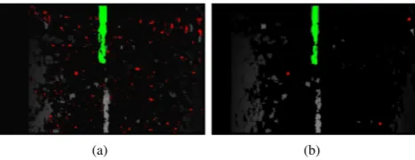
In order to take advantage of the different properties and strengths of the complementary sensors, their measurements are fused into an egocentric multimodal obstacle representation. Figure 2 shows an exemplary scene where a vertical cable is not perceived by the continuously rotating 3D laser scanner but is visible in the disparity map of the stereo cameras.
Figure 1: Our MAV is equipped with a variety of complementary sensors including two stereo camera pairs facing forward and backward.
The contribution of this paper is an evaluation of the suitability of stereo algorithms for obstacle detection on MAVs. We inves-tigate multiple real-time stereo algorithms in combination with different calibration techniques. The major challenge hereby is the modeling of the fisheye lenses, which capture highly radial dis-torted images that need to be rectified in real-time on the onboard computer.
2. RELATED WORK
In recent years, research towards autonomous control of MAVs in complex 3D environments increased considerably. The ability to reliably detect and avoid obstacles is of utmost importance for these tasks. Many research groups equip their MAVs with cameras, but reliable visual detection of obstacles is challenging.
(a) (b) (c) (d)
Figure 2: Fusion of dense stereo measurements and measurements from a continuously rotating laser scanner in an occupancy grid map. a) The raw image of a vertical hanging cable at3 mdistance. b) A dense disparity map showing the detection of the cable. c) A horizontal cut through the occupancy grid map with laser measurements only. d) The grid map after fusing with the stereo measurements. The obstacle is circled blue, whereas the position of the MAV is circled red. White cells correspond to free space, black cells to occupied space, and gray cells to unknown space.
perspectives. Therefore, stereo cameras are used to estimate depth instantaneously, although onboard computation of dense stereo is challenging and necessitates ample processing power.
To cope with the high computational requirements special purpose hardware can be used to calculate the disparity image (Oleynikova et al., 2015). Another recent approach handles the computational limitations by estimating disparities only at a single depth (Barry and Tedrake, 2015).
In (Heng et al., 2011) a quadrotor is equipped with two stereo cam-era pairs to estimate an occupancy grid map for obstacle avoidance. They maintain the output of the OpenCV implementation of the block matching algorithm as 3D point clouds in a 3D occupancy map.
For a more reliable state estimation, cameras are often used in combination with an IMU. With this minimal sensor setup, MAVs are able for autonomous vision-based navigation indoors and out-doors (Schmid et al., 2014). Other groups use the output from stereo matching algorithms as input to visual odometry and offline visual SLAM for autonomous mapping and exploration with a MAV (Fraundorfer et al., 2012).
The majority of these setups use cameras with a small field of view (FOV) less than130◦, so that the general pinhole camera model can be applied. Only limited work has been proposed for the use with fisheye lenses. For example (H¨ane et al., 2014) use fisheye stereo cameras, which are mounted on a car and on an AscTec Firefly quadcopter, to create dense maps of the environment by using an adapted camera projection model. Dense disparity maps are computed in real-time on a modern GPU using an adapted Plane-Sweep.
For the computation of disparity maps from stereo cameras a variety of stereo algorithms exists, which can be classified into local, global, semi-global, and seed-and-grow methods (Scharstein et al., 2001).
Local methods have the advantage that they are fast to compute, but they are in most cases not able to retrieve a dense represen-tation of the scene. Representatives of local methods are, e.g., Block Matching (Szeliski and Scharstein, 2002), Adaptive Win-dows (Kanade and Okutomi, 1991), (Yoon and Kweon, 2006) and Plane-Sweep (Collins, 1996), (Gallup et al., 2007). They often use
cost functions measuring the similarity over local image patches, like the sum of squared distances (SSD), the sum of absolute dis-tances (SAD) or the normalized cross-correlation (NCC). One challenge of local methods is the choice of the window size: if chosen too small or too large, problems with finding the right corresponding patch arise, because either not enough information is integrated or irrelevant image parts are considered. Especially in image regions with low texture, local methods often fail due to their use of only local similarity.
On the other hand, global methods compute a disparity distribu-tion over all pixels by minimizing a global 2D energy funcdistribu-tion— generally consisting of a data fitting term and a smoothness term. Since they search for a global minimization, which finds a cor-respondence for every pixel, they are able to compute a dense disparity map. In most cases, this optimization is NP-hard—so the global methods need much more resources and computation time than local methods. Popular approximations are Graph Cuts (Kol-mogorov and Zabih, 2001), Belief Propagation (Felzenszwalb and Huttenlocher, 2004), or Variational Methods (Kosov et al., 2009).
Semi-global methods, e.g. (Hirschm¨uller, 2008), try to find a balance between global energy minimization and low computation time by combining the local correspondence search with several 1D global energy functions along scan-lines. Another possibility for finding stereo correspondences are so-called Seed-and-Grow methods (Cech and Sara, 2007), (Kostkov, 2003). Starting from random seeds, disparities are grown.
For our task, we focus on algorithms which run in real-time and, in the best case, compute a dense disparity map. We compare representatives of local, semi-global and global methods which are implemented in OpenCV (Bradski, 2000) as well as a prob-abilistic approach available as ROS1 package. A drawback of the usage of these algorithms for our task is that they were not designed for fisheye lenses. Therefore we need to evaluate their suitability for visual obstacle detection with fisheye stereo. As all methods need rectified image pairs, we evaluate them together with different available camera calibration methods. We focus on the OpenCV stereo calibration available in ROS as well as a stereo calibration, which uses a camera model especially designed for fisheye lenses (Abraham and Foerstner, 2005).
1
(a) (b)
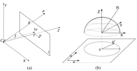
Figure 3: a) Pinhole camera model. b) Fisheye camera model.
3. CAMERA CALIBRATION
The main goal of the calibration of our cameras is to rectify the stereo images, so that corresponding epipolar lines lie in the same image rows. We compare two different models: the pinhole cam-era model, which is widely used as basic camcam-era model, and the epipolar equi-distant model suited well for fisheye lenses.
3.1 PINHOLE MODEL
We make use of the available stereo calibration in ROS, which implements the OpenCV camera calibration based on the Mat-lab calibration tool by Bouguet2and on the calibration technique by (Zhang, 2000). It automatically detects the calibration object, a 2D-checker board, presented to the stereo cameras and estimates the intrinsic and extrinsic parameters of the stereo setup. The un-derlying camera model is the pinhole camera model, illustrated in Fig. 3(a), projecting a 3D point(X, Y, Z)T
is the principal point, that is usually at the image center. For modeling the lens distortion, an additional transforma-tion from distorted image coordinates(u′, v′)T
The distortion coefficientsk1, ..., k6model the radial distortion andp1, p2the tangential distortion. We will evaluate how well this calibration can be applied to model our fisheye stereo setup.
3.2 EPIPOLAR EQUI-DISTANT MODEL
As a second calibration method, we employ the epipolar equi-distant model for fisheye cameras (Abraham and Foerstner, 2005). This model describes the projection of a spherical image onto a plane as shown in Fig. 3(b). In this model, a slightly different projection function is used:
2
Calibration Toolbox, www.vision.caltech.edu/bouguetj/calib doc
Table 1: Overview of the four different calibrations we evaluated.
Name Distortion model Rectification on
Physical Physical (A1, A2) Sphere
Chebychev Chebychev (3rd degree) Sphere
Planar Physical (A1, A2) Plane
OpenCV Pinhole Plane
For modeling the lens distortion, two different approaches are eval-uated: (1) using physical-based polynomials or (2) using Cheby-chev polynomials. Both methods are described in (Abraham and Foerstner, 2005). For the rectification of a stereo camera system, one has the possibility to choose between the projection onto a plane or onto a sphere with epipolar lines.
An overview of the different calibration models that we evaluate is given in Table 1.
4. STEREO ALGORITHMS
For the selection of different state-of-the-art stereo algorithms, which are publicly available and ready to use, we search for meth-ods that find correspondences in real-time. We select different algorithms from local, semi-global, global, and probabilistic types. In addition to the runtime, we evaluate the amount of noise and speckles in the resulting disparity maps.
A very popular local correspondence algorithm is Block Match-ing (BM) (Konolige, 1997), computMatch-ing stereo matches that min-imize the SAD over a local neighborhood. Similar to this, Semi Global Block Matching (SGBM), based on Semi-Global Match-ing (Hirschm¨uller, 2008), is available in OpenCV, which com-bines a SAD-based local cost-function and a smoothness-term in a global energy function. In contrast to these more or less local methods, Variational Matching (VAR) (Kosov et al., 2009) is used as a global algorithm to minimize an energy functional over all pixels. A probabilistic approach for stereo matching is Efficient Large-Scale Stereo Matching (ELAS) (Geiger et al., 2010). By using a triangulation over so-called support points, which can be robustly matched between the two views, a prior for the dispar-ity search is computed and Bayes’ law is applied to compute a MAP-estimate for the remaining pixel, yielding a dense disparity image.
We tested various parametrizations of the different algorithms to minimize noise and wrong correspondences. For all algorithms, we used a maximal disparity range of 100px, leading to a detection of obstacles at distances larger than∼50 cm:
Z =f B
d =
256px·20 cm
100px = 51.2 cm. (4)
employ the Tichonov Penalization which enforces linear smooth-ness over the disparity distribution. ELAS already comes with different parameter presets, which we only modify slightly for our needs: Also here, we set the disparity to 100px and enable the adaptive mean filter.
5. EXPERIMENTS AND RESULTS
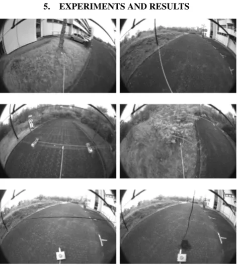
Figure 4: We evaluated the stereo algorithms on five different obstacles with challenging diameters. Top row: Tree (25 cm), street light pole (12 cm). Middle row: Site fence (0.2 cm-4 cm), vegetation. Bottom row: Horizontal and vertical cables (1 cm).
For evaluation, we repeatedly measured the distances from the MAV to five different obstacles discretized in1 msteps from1 m to10 m. As shown in Fig. 4, we selected natural urban obsta-cles with different diameters: a tree (25 cm), a street light pole (12 cm), a site fence (0.2 cm–4 cm), vegetation, and a power cable (1 cm), spanned vertically and horizontally. Particularly difficult to detect are the obstacles with very small diameter and the horizontal cable. The MAV was fixed in height for better com-parison. We used manual and laser scan measurements as ground truth. In total, we recorded 132 datasets with an image resolution of 752×480 pixels.
All computations have been carried out on an Intel Core i7 CPU with 2.2 Ghz. The recorded images have been rectified using the four different calibrations, which were estimated beforehand as described in Section 3. When rectifying the images to a plane, a part of the recorded scene—visible in the raw image—is cut off due to the geometry of the fisheye images. In consequence, the information gained by using a wide FOV is lost in the undistortion step where we project the spherical image onto a plane. After-wards, the disparity maps are generated by the stereo matching algorithms. For evaluation, we manually annotate a pixel mask for every object by labeling pixels that belong to the obstacle.
An example of this processing pipeline can be seen in Fig. 5. The captured fisheye image is rectified using Chebychev calibration and the disparity map is computed by ELAS.
We focus on the following aspects for the evaluation of the suit-ability of the chosen stereo algorithms:
Table 2: Averaged runtimes and densities of the stereo algorithms.
BM SGBM ELAS VAR
fps 19.44 13.55 11.53 7.98
Runtime (ms) 51.44 73.80 86.73 125.31
Density 25.44% 39.55% 84.8% 99.45%
Times measured on an Intel Core i7 processor with 2.2 GHz.
• Runtime: How computational intensive is the algorithm?
• Density: How dense is the disparity map?
• Sensitivity: Does the algorithm detect the obstacle?
• Accuracy: How accurate is the computed disparity?
• Calibration: How does the calibration affect the result?
5.1 RUNTIME AND DENSITY
To autonomously avoid obstacles, it is of utmost importance that the MAV is able to detect the obstacle in real-time. For evaluating the computational costs, we average the runtime of the different algorithms over all available data. Table 2 shows the runtimes measured in ms and frames per second (fps). The density of the computed disparity map is also listed, since it correlates with the runtime. The less points for disparity computation are used, the faster the map can be computed. We aim for fast and dense algorithms, to perceive as much depth points as possible from the scene. It can be clearly seen that the local BM algorithm excels in terms of speed with 19.44 fps, but estimates disparity only for about 25% of the image. On the other hand, VAR as a global method is able to construct a dense disparity map with 99.45% coverage, but is the slowest of the four methods. ELAS makes a very good trade-off between fast computation and the density of its disparity map, yielding a comparatively dense map (84.8%) at 11 fps.
5.2 DETECTION SENSITIVITY AND DISTANCE ERROR
For reliable navigation of autonomous MAVs, it is necessary that the obstacles in the close vicinity are detected. We evaluate the detection in terms of a hit rateS, which represents the rate of successfully detected obstacle points:
S= true positives
true positives + false negatives. (5)
Ideally,Sshould be 1, meaning all disparity measurements be-longing to the obstacle have been computed. In order to calculate this hit rate, we differentiate pixels belonging to the obstacle from the background pixels by using the manually labeled pixel mask and neglect pixels not belonging to the obstacle. These remaining pixels contribute to the detection sensitivity as depth estimates. In Fig. 5(d) the contributing pixels are colored green.
Fig. 6 shows that obstacles with larger diameter have a higher detection rate than obstacles with a smaller diameter, e.g., like the cable. Furthermore, it makes significant difference if the cable is vertically or horizontally spanned. Due to the correspon-dence search along horizontal epipolar lines and the homogeneous texture of the cable, it is not possible for the algorithms in our evaluation to find correspondences for the horizontal spanned ca-ble. While BM and SGBM perform poorly on the cable for both orientations, ELAS and VAR at least have a high detection rate
0% 20% 40% 60% 80% 100%
1m 2m 3m 4m 5m 6m 7m 8m 9m 10m
Detection se
nsitivity
Distance
BM ELAS SGBM VAR
(a) Detection sensitivity of the street light pole
0% 20% 40% 60% 80% 100%
1m 2m 3m 4m 5m 6m 7m 8m 9m 10m
Detection se
nsitivity
Distance
(b) Detection sensitivity of the vertical cable
0% 20% 40% 60% 80% 100%
1m 2m 3m 4m 5m 6m 7m 8m 9m 10m
Detection se
nsitivity
Distance
(c) Detection sensitivity of the horizontal cable
Figure 6: Detection rates of the obstacles with different diameter. While the street light pole has a high hit rate the horizontal cable is hard to detect.
for the vertical spanned cable. None of the algorithms was able to detect the site fence reliably.
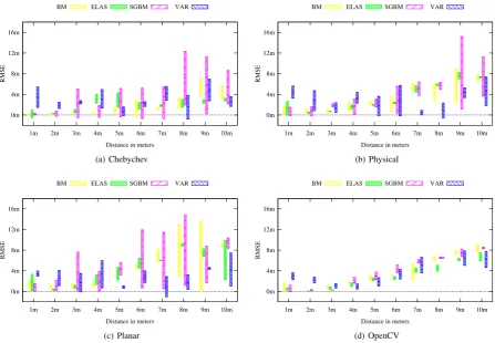
Similarly, we also evaluated the accuracy of the distance estimated to obstacles. To this end, we computed the root-mean-squared er-ror (RMSE) between the estimated distances and the ones obtained from the manual measurements and laser scans. We compute the average distance of all measurements belonging to the obstacle, which are determined by comparing them with the manually la-beled image mask. The error for obstacles that are difficult to detect is in general higher than for those that are easily detected due to their larger diameter. This can be observed in the direct comparison of the detections of the street light pole in Fig. 8 and the vertical cable in Fig. 9.
(a) (b)
Figure 7: Disparity images of BM rectified using Chebychev calibration. False positives are colored red and the obstacle is overlayed with green. With the default settings shown in (a) the disparity map suffers from noisy estimates and speckles. (b) shows the resulting map after applying the speckle filter, resulting in less false positive measurements. The experiments showed that with increasing distance the number of speckles further increases.
Although, the error increases with the distance, the errors of the epipolar equi-distant models grow slower as with the projections onto a plane, For example, with the OpenCV calibration, the error at5 mdistance to the street light pole is3 m, which is significantly higher than the errors of the Chebychev calibration (RMSE below 1m). In comparison to the other algorithms, the estimated depths from ELAS show the lowest variance even at far distances. Besides that, the estimated disparity map from BM, SGBM and VAR are affected by outliers, especially with increasing distance. In all datasets, ELAS excels in terms of error and variance, which can be explained by its underlying probabilistic approach based on strong a-priori knowledge. In contrast, the block matching algorithms suffer from false positives also called speckles in the disparity images. While ELAS and VAR show no false positives at near distances to the obstacle, the disparity images of BM and SGBM include 0.1% (241px) and 1.1% (3976px) false positives at3 m distance to the street light pole.
Since the default setting of the speckle filter results in a high amount of speckles, we increase the window size of the filter. In our experiments a window size of 40px showed best results, i.e., less speckles in the disparity image. Still, a few speckles remain, which would lead to wrong restrictions in the available free space. The impact of the speckle filter for the block matching algorithms is shown in Fig. 7.
While the high variance of BM and SGBM can be explained by the speckles in the disparity image, the variance of VAR is influenced by the so-calledfilling-in-effect, which is typical for global methods. The disparities of image regions where no depth estimate can be computed are approximated from neighboring estimates.
5.3 CALIBRATION
In Fig. 8, we already observed the error of the measurements of a street light pole with different calibrations. In terms of accuracy, the calibration with Chebychev polynomials achieves the best results. Up to5 m, variance and error increase slowly compared to the other calibration methods. This behavior can also be observed at the detection of the other obstacles. For all obstacles—except for the horizontal cable and the site fence where all methods fail— the Chebychev calibration shows the best results. Furthermore, the results show that the different algorithms work better with different calibration methods. For example, ELAS has a lower error in combination with the Chebychev calibration, while the
other algorithms show best results with the Physical and OpenCV calibration.
Moreover, when using the OpenCV calibration, all algorithms have problems finding correspondences in the image corners. This can be explained by the greater distortion resulting from the stan-dard lens distortion model used by OpenCV.
A further drawback of the methods which rectify onto a plane is that a significant part of the image cannot be used. Our exper-iments showed, that obstacles that were positioned at an angle larger than45◦to the optical camera axis are not visible any longer in the rectified image. This prevents omnidirectional obstacle per-ception.
In contrast to the calibration methods that rectify the image on a plane, the equi-distant calibrations were designed for the rectifica-tion of images captured with fisheye lenses, and are able to find correspondences in the image corners.
6. CONCLUSION
We evaluated the suitability of four different state-of-the-art stereo algorithms for reliable obstacle detection on images from stereo cameras with fisheye lenses. In order to deal with the higher dis-tortion of the fisheye lenses, we used different calibration methods to model the lens distortion and to rectify the stereo images. Over-all, all algorithms were able to detect sufficient large obstacles (10cm), although they were not designed for images with such high distortions.
Since the epipolar equi-distant calibrations are designed for fisheye lenses and retain more image information, they are better suitable for the task of omnidirectional obstacle perception with stereo cameras. At close distances, the stereo algorithms have an error below1 m. Obstacles with sufficient diameter could be detected reliably up to10 mwith an average error below3 m. On the other hand, we experienced problems with the detection of obstacles that have a very small diameter, e.g., the site fence (0.2 cm–4 cm). None of the evaluated stereo algorithms could detect it reliably. Likewise, the detection of the cable was very challenging. While the vertical spanned cable could be detected up to5 mby ELAS, the detection of the horizontal spanned cable failed. This is an inherent problem caused by the horizontal baseline of the cameras. To reliably detect cables in all orientations, multi-camera depth estimation is necessary.
0m 4m 8m 12m 16m
1m 2m 3m 4m 5m 6m 7m 8m 9m 10m
RMSE
Distances in meters
BM ELAS SGBM VAR
(a) Chebychev
0m 4m 8m 12m 16m
1m 2m 3m 4m 5m 6m 7m 8m 9m 10m
RMSE
Distances in meters
BM ELAS SGBM VAR
(b) Physical
0m 4m 8m 12m 16m
1m 2m 3m 4m 5m 6m 7m 8m 9m 10m
RMSE
Distances in meters
BM ELAS SGBM VAR
(c) Planar
0m 4m 8m 12m 16m
1m 2m 3m 4m 5m 6m 7m 8m 9m 10m
RMSE
Distances in meters
BM ELAS SGBM VAR
(d) OpenCV
Figure 8: RMSE and corresponding variance of the depth measurements of the street light pole under different calibrations. Error and variance are in general increasing with the distance.
0m 4m 8m 12m 16m
1m 2m 3m 4m 5m 6m 7m 8m 9m 10m
RMSE
Distance in meters
BM ELAS SGBM VAR
(a) Chebychev
0m 4m 8m 12m 16m
1m 2m 3m 4m 5m 6m 7m 8m 9m 10m
RMSE
Distance in meters
BM ELAS SGBM VAR
(b) Physical
0m 4m 8m 12m 16m
1m 2m 3m 4m 5m 6m 7m 8m 9m 10m
RMSE
Distance in meters
BM ELAS SGBM VAR
(c) Planar
0m 4m 8m 12m 16m
1m 2m 3m 4m 5m 6m 7m 8m 9m 10m
RMSE
Distance in meters
BM ELAS SGBM VAR
(d) OpenCV
ACKNOWLEDGMENTS
This work has been supported partially by grant BE 2556/7 of German Research Foundation (DFG) and the German BMWi Autonomics for Industry 4.0 project InventAIRy.
REFERENCES
Abraham, S. and Foerstner, W., 2005. Fish-eye-stereo calibration and epipolar rectification. ISPRS Journal of Photogrammetry and Remote Sensing 59(5), pp. 278–288.
Barry, A. J. and Tedrake, R., 2015. Pushbroom stereo for high-speed navigation in cluttered environments. In: Proc. of the IEEE Int. Conference on Robotics and Automation (ICRA).
Bradski, G., 2000. Opencv library. Dr. Dobb’s Journal of Software Tools.
Cech, J. and Sara, R., 2007. Efficient sampling of disparity space for fast and accurate matching. In: Computer Vision and Pattern Recognition (CVPR), IEEE Conference on, pp. 1–8.
Collins, R., 1996. A space-sweep approach to true multi-image matching. In: Computer Vision and Pattern Recognition (CVPR), IEEE Conference on, pp. 358–363.
Droeschel, D., Holz, D. and Behnke, S., 2014. Omnidirectional perception for lightweight MAVs using a continuously rotating 3D laser scanner. Photogrammetrie-Fernerkundung-Geoinformation (5), pp. 451–464.
Droeschel, D., Nieuwenhuisen, M., Beul, M., Holz, D., St¨uckler, J. and Behnke, S., 2015. Multi-layered mapping and navigation for autonomous micro aerial vehicles. Journal of Field Robotics.
Felzenszwalb, P. and Huttenlocher, D., 2004. Efficient belief propagation for early vision. In: Computer Vision and Pattern Recognition (CVPR), IEEE Conference on, Vol. 1, pp. I–261–I– 268 Vol.1.
Fraundorfer, F., Heng, L., Honegger, D., Lee, G., Meier, L., Tan-skanen, P. and Pollefeys, M., 2012. Vision-based autonomous mapping and exploration using a quadrotor mav. In: Proc. of the IEEE/RSJ Int. Conference on Intelligent Robots and Systems (IROS).
Gallup, D., Frahm, J.-M., Mordohai, P., Yang, Q. and Pollefeys, M., 2007. Real-time plane-sweeping stereo with multiple sweep-ing directions. In: Computer Vision and Pattern Recognition (CVPR), IEEE Conference on.
Geiger, A., Roser, M. and Urtasun, R., 2010. Efficient large-scale stereo matching. In: Asian Conference on Computer Vision (ACCV).
H¨ane, C., Heng, L., Lee, G. H., Sizov, A. and Pollefeys, M., 2014. Real-time direct dense matching on fisheye images using plane-sweeping stereo. In: 2nd International Conference on 3D Vision, 3DV 2014, Tokyo, Japan, December 8-11, 2014, pp. 57–64.
Heng, L., Meier, L., Tanskanen, P., Fraundorfer, F. and Pollefeys, M., 2011. Autonomous obstacle avoidance and maneuvering on a vision-guided MAV using on-board processing. In: Proc. of the IEEE Int. Conference on Robotics and Automation (ICRA), pp. 2472–2477.
Hirschm¨uller, H., 2008. Stereo processing by semiglobal matching and mutual information. Pattern Analysis and Machine Intelli-gence, IEEE Transactions on 30(2), pp. 328–341.
Kanade, T. and Okutomi, M., 1991. A stereo matching algorithm with an adaptive window: Theory and experiment. In: Proc. of the IEEE Int. Conference on Robotics and Automation (ICRA), Vol. 2, pp. 1088–1095.
Kolmogorov, V. and Zabih, R., 2001. Computing visual corre-spondence with occlusions using graph cuts. In: Computer Vision (ICCV), Eighth IEEE International Conference on, Vol. 2, pp. 508– 515.
Konolige, K., 1997. Small vision system: Hardware and imple-mentation. In: International Symposium of Robotics Research (ISRR), pp. 111–116.
Kosov, S., Thormaehlen, T. and Seidel, H.-P., 2009. Accurate real-time disparity estimation with variational methods. In: Pro-ceedings of the 5th International Symposium on Advances in Visual Computing: Part I, ISVC, Springer, pp. 796–807.
Kostkov, J., 2003. Stratified dense matching for stereopsis in complex scenes. In: British Machine Vision Conference (BMVC), pp. 339–348.
Oleynikova, H., Honegger, D. and Pollefeys, M., 2015. Reactive avoidance using embedded stereo vision for mav flight. In: Proc. of the IEEE Int. Conference on Robotics and Automation (ICRA).
Ross, S., Melik-Barkhudarov, N., Shankar, K. S., Wendel, A., Dey, D., Bagnell, J. A. and Hebert, M., 2013. Learning monocular reactive uav control in cluttered natural environments. In: Proc. of the IEEE Int. Conference on Robotics and Automation (ICRA), IEEE, pp. 1765–1772.
Scharstein, D., Szeliski, R. and Zabih, R., 2001. A taxonomy and evaluation of dense two-frame stereo correspondence algorithms. In: Stereo and Multi-Baseline Vision (SMBV), IEEE Workshop on, pp. 131–140.
Schmid, K., Lutz, P., Tomic, T., Mair, E. and Hirschm¨uller, H., 2014. Autonomous vision-based micro air vehicle for indoor and outdoor navigation. Journal of Field Robotics 31(4), pp. 537–570.
Szeliski, R. and Scharstein, D., 2002. Symmetric sub-pixel stereo matching. In: 7th European Conference on Computer Vision (ECCV), pp. 525–540.
Yoon, K.-J. and Kweon, I.-S., 2006. Adaptive support-weight ap-proach for correspondence search. Pattern Analysis and Machine Intelligence, IEEE Transactions on 28(4), pp. 650–656.