Rule-dynamical generalization of McCulloch – Pitts neuron
networks
Yoshinori Nagai
a,b,*, Yoji Aizawa
caCenter for Information Science,School of Political and Economic Sciences,Kokushikan Uni6ersity,4-28-1Setagaya,
Setagaya-ku,Tokyo154-8515,Japan
bDepartment of Applied Mathematics,Research School of Physical Sciences and Engineering,Australian National Uni6ersity,
Canberra,ACT0200,Australia
cDepartment of Applied Physics,School of Science and Engineering,Waseda Uni6ersity,3-4-1Okubo,Shinjuku-ku,
Tokyo169-8555, Japan
Abstract
A new aspect for neuronal networks is presented. The aspect is based on the concept of ruledynamics which was originally proposed by one of the authors, Aizawa. The concept of ruledynamics were modeled on the two states
cellular automata of neighborhood-three (CA2
3). A brief review of ruledynamics is also presented, because most
publications of the authors so far have been in Japanese. Our concise assertion in the present paper is that a neuronal network realizes a kind of ruledynamics. This assertion is a speculation on the comparison of McCulloch – Pitts
neuron networks with ruledynamics on CA2
3. A trial is originally shown to demonstrate that a McCulloch – Pitts
neuron network can be imitated by an extended version of ruledynamics on CA2
3. © 2000 Elsevier Science Ireland
Ltd. All rights reserved.
Keywords:Ruledynamics; Rule space; Cellular automata; McCulloch – Pitts neuron network; Threshold change
www.elsevier.com/locate/biosystems
1. Introduction
Aizawa proposed the concept of a new paradigm for an extended dynamics, that was called ‘‘Ruledynamics’’, Aizawa and Nagai (1987). We actually realized a ruledynamics apply-ing the concept for the two states cellular au-tomata of neighborhood-three which was intensively investigated by Wolfram (1983, 1986). Then, we constructed a rule-dynamical system on
the two states cellular automata of neighborhood-three (CA2
3), based on the work by Aizawa and
Nishikawa (1986). They asserted that the pattern dynamics of CA2
3, except for travelling patterns,
can be reproduced by 32 rules which are given by a combination of the five fundamental rules. Then, we made a new kind of two states cellular automata of neighborhood-three (CA2
3) in which
the rule to govern the change of each cell state also varies in some manner, step-by-step, over time. We designed four types of rule change, Aizawa and Nagai (1987), namely:
* Corresponding author.
1. the rule is changed by an arbitrary external function of time;
2. the rule change is changed by using the aver-age activity of a cell array and a threshold for each rule (for example, a rule is switched, or reversed to its opposite, on the average activity over the threshold);
3. hybrid of manners 1 and 2;
4. multigate method in which switch-on regions and switch-off regions are prepared for a rule with respect to the average activity.
We call this kind of CA2
3 ‘‘ruledynamics on
CA2
3’’. We also call a series of temporal
develop-ment of cell states of CA2
3 a pattern dynamics.
In the generalized sense, the ruledynamics is the temporal change of rules which governs the tem-poral development of quantities in a system. It is an expandable concept. For ruledynamics on CA2
3, one can see that the change of rules over
time gives rise to more complicated temporal pat-terns, some of which cannot be seen in Wolfram approach to CA2
3. These patterns, however, may
be found out in higher neighborhood cases. The neighborhood referred to here means the con-tributed cells to determine the state of each cell at the next point in time. Then, the ruledynamics on CA2
3 can realized a subgroup of
multi-neighbor-hood cellular automata of two states. Most of our works concerned with ruledynamics were pub-lished in Japanese. A review of the ruledynamics is therefore given in Section 2.
Since the ruledynamics on CA2
3is a model only,
by using a computer program, we sought how the rule switching brings about physically and ob-served what system can actually perform the rule-dynamics. We discovered the physical reality of ruledynamics through the consideration of neural networks consisting of McCulloch – Pitts type neu-rons, each of which is an abstracted nerve cell with two states (firing, resting). The state change of an element in any two-state system can be expressed by a Boolean function. The rule change therefore means making the choice of a Boolean function. This is the same in a McCulloch – Pitts neuron network. The control of rule selection is carried out automatically by the activities of in-hibitory neurons connecting to each other and to excitatory neurons. This is the fundamental
recog-nition of ruledynamics and we understand that the concept of ruledynamics can be applicable to actual neuronal networks in the brain. These points are discussed in Section 3. In our standing point, neuronal cording exists in relationships re-duced from the temporal development of cell ar-ray states.
Although we already knew the equivalence of the ruledynamics on CA2
3 to McCulloch – Pitts
neuron network, Nagai and Aizawa (1995, 1997), it was difficult to derive directly a set of equations of ruledynamics on CA2
3 from those of
McCul-loch – Pitts neuron network. We therefore assert that the ruledynamics on CA2
3 can produce the
same pattern dynamics generated by the McCul-loch – Pitts neuron network. Here, the equivalence of a ruledynamics on CA2
3 to a McCulloch – Pitts
neuron network means that a ruledynamics on CA2
3 reproduces the same relationship of pattern
dynamics generated by a McCulloch – Pitts neuron network. We speculate that an extended ruledy-namics of site-dependent rule change can imitate McCulloch – Pitts neuron networks. An actual demonstration for this speculation is carried out by using a ring form of eight McCulloch – Pitts neurons. These are shown in Section 4.
2. Ruledynamics on two state cellular automata of neighborhood-three
In this section, we provide a concise review of our previous works for ruledynamics on CA2
3and
then we expand the ruledynamics on CA2 3 to the
ruledynamics of site-dependent rule changes. The requirement will be realized when we recreate any binary system by using the ruledynamics on CA2
3.
A ruledynamics was realized on the cellular automata. Following the approach taken in the study by Aizawa and Nishikawa (1986), we ex-tend pattern dynamics of the two states cellular automata of neighborhood-three CA2
3, Wolfram
(1983, 1986), to ruledynamics, Aizawa and Nagai (1987), by changing the coefficients for the combi-nation of basic five rules temporally. Aizawa and Nishikawa concluded that most of temporal pat-terns of cell states on CA2
3 can be reproduced by
combina-tion in a fundamental basis of five rules {g1,g2,g3,
g4,g5}. The fundamental rule basis is the
follow-ing five rules:
g1=f0=Si−1+Si+Si+1, (2.1)
g2=f1=Si−1 · Si+Si · Si+1+Si+1· Si−1,
g
3=f2=Si−1 ·Si · Si+1, g4=p=(Si−Si−1) · (Si−Si+1),
g5=f1 · p (mod 2 for all),
where f0, f1, f2, and p are the notations used in
Aizawa and Nishikawa (1986) and Si takes the
value 0 or 1. The notation to represent the func-tions of rules for CA2
3 is followed as by Aizawa
and Nishikawa (1986). Aizawa and Nishikawa’s rule basis is modified from Wolfram (1983), origi-nally. Wolfram (1986) also presented the represen-tation of rules by Boolean functions. But the simple representation is given by the form of modulo 2. For Aizawa and Nishikawa’s rule ba-sis, only two basic rules become simple Boolean functions. Theg1 is equivalent to the logic
exclu-sive-OR andg3is the logic AND. The other three
are not simple. So, we use the form of modulo 2 for rules of CA2
3.
The ruledynamics becomes the temporal devel-opment of each element cell state in the array ofn
cells given by the following recurrence equation:
Si(t+1)=% k
ok(t) ·gk(Si−1(t),Si(t),Si+1(t))
(mod2), (2.2)
where ok(t) denotes the coefficient for kth basis
rule at time t and changes the value 1 or 0 temporally. Self-sustaining pattern development in the ruledynamics appears when a quantity con-cerned with pattern is fed back to coefficients {ok(t)}. An example is shown in Fig. 1 in which
the coefficients of fundamental rules are deter-mined using the average activity of the cell array at the previous time. The temporal development of ith cell state for this case is expressed as follows, Aizawa and Nagai (1989):
Si(t+1)=% k
u(hk(Sit−Tk)
· gk(Si−1(t),Si(t),Si+1(t)) (mod2),
(2.3)
where BSi\t denotes the average activity at
timet, Tkmeans a switching threshold for rulek,
u(x) is the Heaviside step function,hksignifies the
sign for switching manner, namely, +1 denotes switch-on if BSi\t takes a value greater than
the threshold Tk and −1 switch-on if BSi\t
takes lower than the threshold Tk. This type of
ruledynamics on CA32 has the average activity
Fig. 1. An example of the ruledynamics on CA32: (a) temporal pattern of cell states, (b) temporal change of rules and (c) time course
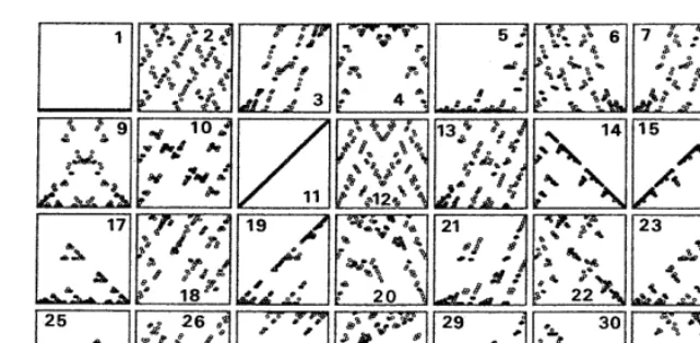
Fig. 2. Relationship between state vectors at timetandt+1 for CA32. System size is 7. Aizawa – Nishikawa 32 rules are depicted.
synchronization behavior investigated by Kim and Aizawa (1999). The average synchronization implies that a given temporal rule change attracts the temporal pattern changes of cell states for any initial configuration of cell states in the average activity sense. In other words, the pattern dynam-ics for the given temporal rule change become similar to each other. This is a kind of robustness of the ruledynamics on CA3
2
. Usually, the time course of average activity behaves like that of electro encepharo gram (EEG), Aizawa and Na-gai (1989) as shown in Fig. 1c. The ruledynamics brings a large scale fluctuation in the temporal behavior of the average activities if rule switching occurs at a certain value of the average activity, since each rule has the characteristic that the average activity for considered rule converges to a certain value within normal fluctuation, Gutowitz et al., 1987.
In order to see any two state system can be imitated by a certain ruledynamics, we extend the rule-change method, making it more general. The most generalized case is described by following expression, i.e.,
Si(t+1)=fi,t(Si−1(t),Si(t),Si+1(t)) (mod 2),
(2.4) wherefi,t{f0,f1,f2,...,fm} is a rule in a rule space
that is selected for each site of the cell array and each step of time development. In the general situation, it is suitable to describe the temporal
development of the system using the state vector of the systemS(t)=(S1(t),S2(t),...,Sn(t)) at time
t. The time development of the state vector is given by the following formal recurrence equa-tion, namely:
S(t+1)=Ftt+1(S(t)), (2.5)
whereFtt+1is the formal expression of a global
rule. The global rule means the relationship be-tween the states of a whole system from time tto time t+1. The assignment of state vectors to rational numbers yields a representation of the global rule. The examples of global relation of state vectors at timetandt+1 are shown in Fig. 2, where the rational number assignment is taken as j(t)=S2iS
i(t).
3. Rule-dynamical aspect of McCulloch – Pitts neuron network
Si(t+1)=u
%WijSj(t)−Ti, (3.1)whereSi(t) is the state ofith neuron at timet,Wij
denotes the connection weight fromjth neuron to
ith neuron,Timeans the threshold ofith neuron,
and u(...) signifies the Heaviside step function, i.e.,u(x)=1, for x`0, and u(x)=0 for xB0.
Firstly, we consider a simple network whose temporal development is described by the follow-ing directly equivalent equation to CA2
3, namely,
Si(t+1)=u(Si−1(t)+Si(t)+Si+1(t)−Ti).
(3.2) It is obvious from Eq. (3.2) that Boolean func-tion like relafunc-tion betweenSi(t +1) and (Si−1(t),
Si(t),Si−1(t)) is changed when the thresholdTiis
varied. The result of Eq. (3.2) for the threshold values is expressed as follows:
Si(t+1)=1 forTi 0, Si(t+1)
where Boolean logics NOT, OR, and AND are reprented by , OR, and AND, respectively. The fact referred to here was investigated by many researchers for more general case described by the equation similar to Eq. (3.1)(Hu, 1965; Lewis II and Coates, 1967; Sheng, 1969; Muroga, 1971). This research field is Threshold logic. In the dif-ferent value case of connection weights {Wij},
many more types of Boolean functions appear in the relationship between Si(t+1) and (Si−1(t),
Si(t),Si+1(t)) than the simple case, as seen in the
textbook by Muroga (1971). Hence, it is obvious that the change of threshold value brings a change in the Boolean relationship. Since the temporal development of state in a McCulloch – Pitts neuron network is governed by threshold logic processes, the rule-dynamical property of
McCul-loch – Pitts neuron network realizes the change of threshold over the time.
To consider the rule-dynamical property of Mc-Culloch – Pitts neuron network, we rewrite the Eq. (3.1) for the temporal development of McCul-loch – Pitts neuron network as follows:
Si
W++the connection weight from excitatory
neu-ron to excitatory one,W− +that from excitatory
neuron to inhibitory one, W+ −
the absolute value of connection weight from inhibitory neu-ron to excitatory one, and W−− that from
inhibitory neuron to inhibitory neuron. The rewritten equations explicitly express the temporal change of the threshold caused by the activities of inhibitory neurons. Therefore, it is obvious that the McCulloch – Pitts neuron network becomes a kind of rule-dynamical system proposed by us if the network has inhibitory neurons in connections.
neuronal network, the rule corresponds to the orbital manifold in the phase space, the shape of which is deformed by the stimulus current. A neuronal activity is just an orbit on the manifold. The change in the manifold shape therefore produces a change of orbit, namely, varies temporal shape of action potential. In this sense, we can establish the concept of rule for the electric potential activities in real nervous systems.
4. Correspondence of ruledynamics on two state cellular automata of neighborhood-three to McCulloch – Pitts neuron network
In this section, we consider how to realize the complete reproduction of pattern dynamics by the ruledynamics on CA3
2for any temporal pattern of
cell states appearing in the McCulloch – Pitts neu-ron network. The method will be applicable for any system of two states. As seen from the Eq. (3.1) for temporal development of cell states in McCulloch – Pitts neuron network, it is difficult to reduce the equation in the form of Eq. (2.2) or Eq. (2.3) from Eq. (3.1). If we restrict the case of uniform weight connections, the McCulloch – Pitts neuron network is equivalent to multi-neighbor-hood two states cellular automata. Generally, the McCulloch – Pitts neuron network has non-uni-form connection weights so that direct derivation of cellular automata type equations from Eq. (3.1) is impossible. We therefore take another strategy to interpret the McCulloch – Pitts neuron network as a ruledynamics on CA32.
The new strategy utilizes the relationship be-tween state vectors at time t and t+1. In other words, we regard a ruledynamics on CA32 as the
McCulloch – Pitts neuron network, if the relation-ship between state vectors according to the rule-dynamics on CA3
2
gives the same temporal development of cell states of the McCulloch – Pitts neuron network, except for the difference appear-ing in the transient development of cell states at an early stage of time. If a ruledynamics on CA3 2
presents the exact relation between state vectors at time t and t+1, in which the mapping of each state vector at timetto a state vector at timet+1 is exactly the same as the mapping form given by
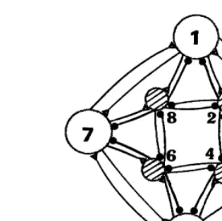
Fig. 3. Neuron connection of ring-net: odd numbers are excitatory neurons and even numbers inhibitory neurons.
the McCulloch – Pitts neuron network, this ruledy-namics on CA3
2 in the property of function does
not differ from the corresponding McCulloch – Pitts neuron network.
Now, we demonstrate the property of ruledy-namics on CA3
2
discussed above, using a simple McCulloch – Pitts neuron network consisting of four excitatory neurons and four inhibitory neu-rons as shown in Fig. 3. We call this a McCul-loch – Pitts neuron network ‘‘ring-net’’. The activity of the ring-net varies against the change of connection weights and proper threshold of each neuron. Connection weights and proper threshold should be regarded as the parameters to see activity change in the ring-net. The ring-net activity can be seen from the relationship between state vectors at time t and t+1. We call this relationship a return map of state vectors. Two examples are shown in Fig. 4 for different parameter values. The complicated feature is seen in the return map of state vectors when the ring-net includes inhibitory neurons. If the ring-ring-net has no inhibitory neurons, namely, has been orga-nized only by excitatory neurons, the return map of state vectors becomes simplified. Only two or four flat dot arrays exist there.
Fig. 4. Relationship between state vectors at timetandt+1 for ring-net. The parameters area,a’:W++=1,W− +=1,
W+ −= −0.8,W−−= −0.72,T+=T−=1,b,b’: W++
=1, W− +=1, W+ −= −0.5, W−−= −0.5, T+=1.2,
T−=0.96.a,bdenote the return map:S(t)S(t+1), anda%,
b%thetth iterated map:S(t)S(t+50).
Fig. 6. Temporal change of relative threshold. The relative threshold includes the effect of inhibitory neuron activities. The cell state changing over time and the temporal change of the relative threshold are depicted for each cell. Only periodic behavior appeared.
cated development of cell states over time. In Fig. 5, we show the temporal development of initial state vectors at a later stage of time by use of the
tth iterated maps. In Fig. 6, we also demonstrate temporal change of threshold discussed in the previous section. The rule change, by the change of relative threshold value, hides behind the tem-poral change of state vector.
We consider the complicated feature of return maps shown in Fig. 4and Fig. 5, based on the fact that the temporal development of each cell state is silent state over time occurs for a significant
num-ber of initial states. In the case shown in Fig. 4(b), almost all initial states undergo a silent state, but a few initial states survive in cyclic developments of cell states. The case in Fig. 4(a) shows that far more initial states survive and form more
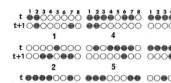
Fig. 7. Ambivalent cases selected in mapping of state vectors. A black circle denotes a firing state and an open white one corresponds to the resting state of a neuron.
(Si−1(t), Si(t), Si+1(t)) and Si(t+1) such as (S,
S%, S¦)0 or 1 at the same time in the same vector components. Fig. 7 shows an example of ambivalent cases of ring-net, where eight circles denote the neurons (the odd number is excitatory neurons and the even number inhibitory neurons). As seen from Fig. 7, ambivalent mappings such as (0,0,0)0 or (0,0,0)1 occurred in a ring-net for all the cases depicted in the figure. The results are summarized in Table 1. If two state vectors have no ambivalence in their relation, the mapping (Si−1, Si, Si+1)Si fits with a rule of CA3
2
. To apply the cellular automata rules for the ambiva-lent mappings, we have to use different assign-ments of rules to the ambivalent mappings. Then, the use of a set of rules {f1,f2,f3,f4,f5,f6,f7,f8}
gives perfect assignment of rules in CA3
2 to any
two states system, where f1...f8 signify the local
rule of each site from time t to time t+1. This method is valid for any ambivalent mapping of binary systems. We knew that two complementary rules is enough to construct a rule set (a rule vector) which can determine any temporal devel-opment of state vectors. Note that two comple-mentary rules satisfy the relation f(Si−1, Si, the complementary rule. For the example of inap-plicable cases on the ring-net, we also show how to organize the rule vector in the Table 1. We chose two complementary rules as fa=g1 and
simple as shown in Fig. 6. The complicated fea-ture of the relation S(initial)S(t) of state vec-tors, i.e., tth iterated map does not infer the complicated development of each cell. Each cell takes one of the states, namely, continually firing over time, silent over time, and periodic firing (alternative excite and rest, three times excite and one rest, one time excite and three times rest). Hence, the complicated feature in thetth iterated map implies that the combined behavior of the cell activities, i.e., periodic firing, all the firing over time and silent, coexists in the nerve cell array. Then, the temporal development of cell state vectors are different from that appearing in each cell.
The difficulty appears when we imitate McCul-loch – Pitts neuron network by ruledynamics on CA3
2, which is an ambivalent relationship between
Table 1
fb=g1, where g1 means that NOT logic is
operated to the ruleg1. The method can formally
be expressed as follows:
S(t+1)=ft·S(t), (4.1)
where ith element is exactly equal to Si(t+1)=
fi,t,(Si−t(t),Si(t),Si+1(t)), (mod 2), with fi,t{fa,
fb}. Within this method, we can construct the
equivalent ruledynamics on CA32to the ring-net or
other McCulloch – Pitts neuron networks.
References
Aizawa, Y., Nagai, Y., 1987. Dynamics on pattern and rule – rule dynamics (in Japanese). Bussei Kenkyu 48, 316 – 320. Aizawa, Y., Nagai, Y., 1989. Rule dynamics and fuzzy attrac-tor: new approach to EEG. In: Takayama, H. (Ed.), Cooperative Dynamics in Complex Physical Systems. Springer, Berlin, pp. 269 – 270.
Aizawa, Y., Nishikawa, I., 1986. Toward the classification of the patterns generated by one-dimensional cell automata. In: Ikegami, G. (Ed.), Dynamical Systems and Nonlinear Oscillations. World Scientific, Singapore, pp. 210 – 222. Gutowitz, H.A., Pitts, W.H., Victor, J.D., Knight, B.W., 1987.
Local structure theory for cellular automata. Physica D28, 18 – 48.
Hayashi, H., Ishizuka, S., Hirakawa, K., 1985. Chaotic re-sponse of the pacemaker neuron. J. Phys. Soc. Jpn. 54, 2337 – 2346.
Hayashi, H., Ishizuka, S., 1992. Chaotic nature of bursting discharges in the onchidium pacemaker neuron. J. Theor. Biol. 156, 269 – 291.
Hu, S.T., 1965. Threshold Logic. University of California Press, Berkeley.
Kim, S.J., Aizawa, Y., 1999. Synchronization Phenomena in Rule Dynamical Systems. Prog. Theor. Phys. 102, 729 – 748.
Lewis II, P.M., Coates, C.L., 1967. Threshold Logic. Wiley, New York.
McCulloch, W.S., Pitts, W.H., 1943. A logical calculus of the idea imminent in neural net. Bull. Math. Biophys. 5, 115 – 133.
Muroga, S., 1971. Threshold Logic and its Application. Wiley-Interscience, New York.
Nagai, Y., Aizawa, Y., 1995. Hierarchical structure and rule-dynamics (in Japanese). Tech. Rep. Inform. Process. IEEJ IP-95-19, 51 – 59.
Nagai, Y., Aizawa,Y., 1997. Equivalence of information pro-cesses between cellular automata and neural network. In: Proc. 1997 Int. Symp. Nonlinear Theory and its Applica-tions (NOLTA 1997), vol. M3C2, pp. 657 – 660.
Sheng, C.L., 1969. Threshold Logic. Ryerson Press, Toronto. Wolfram, S., 1983. Statistical mechanics of cellular automata.
Rev. Mod. Phys. 55, 601 – 644.
Wolfram, S., 1986. Theory and Application of Celluar Au-tomata. World Scientific, Singapore.