RPA pathwise derivative estimation of ruin probabilities
q
Felisa J. Vázquez-Abad
Department of Computer Science and Operations Research, University of Montreal, Montréal, Que., Canada H3C 3J7
Received 1 November 1998; received in revised form 1 March 1999
Abstract
The surplus process of an insurance portfolio is defined as the wealth obtained by the premium payments minus the reimboursements made at the times of claims or accidents. In this paper we address the problem of estimating derivatives of ruin probabilities with respect to the rate of accidents. We study two approaches, one via a regenerative storage process and the other via importance sampling. For both processes we can apply the rare perturbation analysis (RPA) method for sensitivity estimation. We provide computer simulation results. © 2000 Elsevier Science B.V. All rights reserved.
Keywords:Ruin probabilities; Accident; Surplus process
1. Introduction
The surplus process of an insurance portfolio is defined as the wealth obtained by the premium payments minus the reimbursements made at the times of claims. The canonical model for the surplus process is
U (t )=u+ct−
N (t )X
i=1
Yi, t ≥0,
whereN (t )is a Poisson process with ratelthat models the epochs when claims are made and the corresponding
amounts{Yi}are assumed to be i.i.d. random variables with distributionGand meanβ. Premiums are received at
constant ratec. SetTτ =min{t :U (t ) <0}, the ruin probability is
ψ(u, λ)=P{Tτ <∞}.
Ifc ≤ λβ, thenψ(u, λ) = 1 for all initial endowmentu (Gerber, 1979). As a consequence of this result, it is common to assume that premiums satisfyc > λβ, which we will do.
The variant of the model that we consider is given in Gerber (1979), Asmussen (1985), Asmussen and Nielsen (1995). It is assumed that the wealth available is invested at some continuously compounded interest rateδ. The resulting surplus process is of the form:
dU (t )=(c+δU (t ))dt−dS(t ); U (0)=u, (1)
qThis work was completed while the author was on leave at the Department of Electrical and Electronic Engineering, Melbourne University, Australia.
E-mail address:[email protected] (F. J. V´azquez-Abad)
270 F.J. V´azquez-Abad / Insurance: Mathematics and Economics 26 (2000) 269–288
whereS(t )=PN (t )i=1Yiis the compound Poisson process of cumulative claims. Use the notation{Tn, n≥0}as the
event epochs of the processN(t), withT0≡0, and denote byWn=Tn−Tn−1the interarrival times.
Since for general distributionsGthere is no analytical expression for the ruin probability available, one often resorts to simulation techniques. However, estimatingψ(u, λ)via direct simulations of the processU (t )would require estimatingP(A), whereAis a rare event. For paths where ruin is not achieved, we do not have any infallible stopping rule for the simulation.
Section 2 presents two methods for estimatingψ consistently by simulation. The first method uses indirect estimation via the surplus process, a queueing related process for which an overflow probability equals ψ, as will be summarized in Section 2.1 (see Asmussen, 1985; Gerber, 1979; Michaud, 1993). The second method was introduced by Asmussen and Nielsen (1995) for a general framework and it uses importance sampling, a common method for estimation of rare event probabilities, as explained in Bratley et al. (1987), and will be presented in detail in Section 2.2. For the interest model this method prescribes simulating another process where claims follow a non-homogeneous Poisson process with rates that are adapted to the natural filtration of the process. We restate the results of Asmussen and Nielsen (1995) with an independent formulation for a particular claim amount distribution. Three parameters of the model are of importance: the premium rate, the accident rate and the mean claim amount. Lower premiums are more competitive, but might increase the probability of ruin. The sensitivities of the ruin probability to these parameters may therefore provide important information in establishing premiums and evaluating sensitivities to risk. In Vázquez-Abad and Zubieta (2000) the relationships between the derivatives of the ruin probability to each of the three parameters are developed. It is further shown that they may all be expressed in terms of the sensitivity to the accident rateλ, but this may be even more difficult to compute than evaluating the ruin probability itself.
This work focuses on the estimation of the sensitivities ofψ(u, λ)to the arrival rateλusing the RPA method. Section 3 is devoted to the application of RPA to both the storage process and the importance sampling method of Section 2. The phantom RPA method is applied directly to the storage process in Section 2.2.1, using the same techniques as in Brémaud and Vázquez-Abad (1992), but a continuity correction term must be included for the importance sampling method, as discussed in Section 2.2.2. Furthermore, the phantom version of RPA requires extra simulations in this model, which may hinder efficiency. The virtual RPA method of Section 3.2.2 avoids this problem. To our knowledge, this is the first application of the method of Baccelli and Brémaud (1993), which we implement for the non-homogeneous Poisson arrivals model.
Section 4 describes the phantom and virtual estimators and provides the recursion formulas to program these methods efficiently. The simulation results are in Section 5, where functional estimation via the storage process is discussed. Our simulations compare the two estimation methods for the exponential claim distribution, where formulas for ψ and its derivatives are available, thus allowing for a better assessment of the behaviour of the estimators.
2. Estimating the ruin probability
2.1. The storage process
Gerber (1979) shows that the complement of the probability of ruinψ(u)¯ =1−ψ(u)satisfies a renewal equation when the accidents occur according to a Poisson process, namely:
c ∂
∂uψ(u)¯ =λψ(u)−λ
Z u
−∞
¯
ψ(u)dG(y)
with boundary condition limu→∞ψ(u)¯ =1.
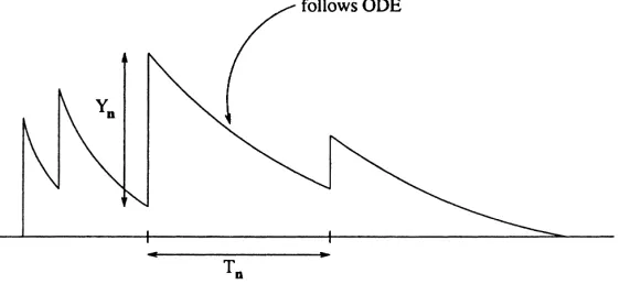
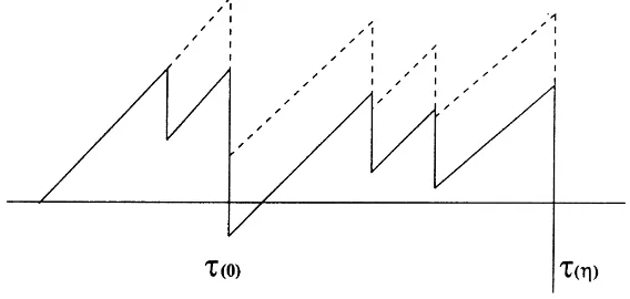
Fig. 1. A typical cycle in a trajectory ofX(t ).
X(t )=dS(t )−(c+δX(t ))+dt; X(0)=x0 (2)
where(x)+≡max(0, x). This process regenerates whenc > λβeven ifδ=0, the stationary measure exists and is unique. In Vázquez-Abad and LeQuoc (2000) the equivalence betweenX(·)and a queueing process is discussed. Asmussen (1985) and Gerber (1979) show that the complement of the overflow probability ofX(·)satisfies the same renewal equation asψ(u)¯ with the same boundary condition, which implies:
ψ(u, λ)= lim
t→∞P{X(t ) > u} =tlim→∞
1
t
N (t )X
n=1
Dn, (3)
whereN(t)is the number of claims received within [0,t) andDnis the total amount of time that the processX(·)
spends above leveluwithin the interval [Tn−1, Tn). As shown in Fig. 1, fort ∈[Tn−1, Tn)the processX(t)follows
an ODE and therefore is given by:
X(Tn−1+s)=
e−δshX(Tn−1)− c δ(e
δs
−1)
i+
,
s∈[0, Wn)X(Tn)=
e−δWn[X(T
n−1)− c
δ(e
δWn−1)]
+
+Yn.
The embedded process{X(Tn);n=0,1, . . .}can be used for discrete event simulation in order to estimate the
ruin probability as well as its sensitivities.
2.2. Importance sampling
2.2.1. The linear model
Consider the linear model (δ =0) for the surplus processU(t), and let
τ =min
(
n:u+cTn ≤ n
X
i=1 Yi
)
. (4)
It is a stopping time and, ifh[(Wi, Yi);i = 1, . . . , τ] = 1{τ <∞}then by definition,E[h] = ψ(u, λ), whereE
denotes expectation with respect to the measure of the process when the accidents occur according to a Poisson process with rateλand the claims are i.i.d.∼G.
The method of importance sampling presented in Siegmund (1976), Asmussen and Nielsen (1995), Bratley et al. (1987), and Ross (1997) is based on a change of measure under which ruin is certain. Letλ0> λand
272 F.J. V´azquez-Abad / Insurance: Mathematics and Economics 26 (2000) 269–288
Letg(y)denote the density ofY1(orP[Y1=y] in the case of discrete claim distributions) and assume thatYi >0
a.s.
Suppose that a processU(t)is simulated, with accidents occurring at a rateλ0and claim amounts following the exponentially tilted distribution:g(y)˜ =Keµyg(y)andK−1=E[eµY], also known as the Esscher transform ofY. Naturally, this can only be well defined if the moment generating function ofYexists on an open interval containing
µ, that is, ifE[eµY]<∞. Otherwise, the method can still be used under a different change of measure and different stability assumptions, as presented in Vázquez-Abad and LeQuoc (2000). Setλ0at a value such that ruin is certain.
By independence of the random variables{Wi, Yi},
whereE˜λ0 denotes expectation under the new measure. Sinceψ(u, λ) =
P
whereSτ =Pτi=1Yi. The term appearing inside the expectation, called the likelihood ratio, is the Radon–Nikodym
derivative of the original measure (restricted to the set{τ <∞}) w.r.t. the new measure. Notice that, by (4),
(λ0−λ)Tτ −
LetRbe the adjustment coefficient of the original process Gerber (1979), defined by the implicit equation
λE[eRY]=λ+Rc. (6)
The condition for certain ruin under the new measure isλ0> cE˜λ0[Y]. It follows from Asmussen and Nielsen (1995)
that under some conditions,λ+Rc> cE˜λ0[Y]. Choosingλ0=λ+Rc, we haveµ=Randλ/K =λE[eRY]=λ0.
Then the likelihood ratio is less than one on the trajectories whereτ <∞, which bounds the variance of the estimator. Otherwise, ifλ+Rc< cE˜λ0[Y], then in order to have certainty of ruin we must chooseλ0> λ+Rc, in which case
it is necessary to assume that the new claim distribution satisfiesE˜λ0[eατ]<∞, forα=lnλ− lnKλ0.
Remark 1. There is an implicit equation relating the moment generating function ofτ, ϕτ(z)=E[ezτ]and that
of the claim distributionϕY(z),given by:ϕτ(z)=ϕY[z/c+λ/c(1−ϕτ(z))].This formula follows from Tackács
argument (see Kleinrock, 1976, pp. 206–216) for the busy periods of anM/G/1queue with accelerated service at rate c. It is therefore possible to verify the existence ofϕτ(z)for some claim distributions.
2.2.2. Interest model
Whenδ >0 in (1), there is not afixedvalueλ0that ensures certainty of ruin under a similar change of measure as
in the linear case. However, a change of measure under which ruin is certain is possible by adjusting the values of the new rate and tilt parameter depending on the current state. That is, at claim numbern, generate the next arrival epochWn+1as an exponential with a different rateλnand generate the claim sizeYn+1under the Esscher transform
with tiltµn, where bothλn, µndepend on the stateU (Tn).
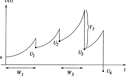
Fig. 2. Continuous processU (t )and embedded process{Un}(dots).
present it for the particular case when the claims are exponentially distributed. Other claim distributions are treated similarly.
Consider the embedded discrete time processUn =U (Tn)(with the obvious abuse of notation), shown in Fig.
2. From (1),U (·)follows the dynamics of an ODE between claims, and then jumps according to the amount of the claim, yielding:
Un+1=UneδWn+1 +c
eδWn+1−1
δ
−Yn+1. (7)
DefineRnas the local adjustment coefficient that satisfies:
λ+(c+δUn)Rn=λE[eRnY],
which for the exponential case reduces toRn=β−1−λ/cn, withcn=c+δUn. Setλn=λ+cnRn=cn/βand
µn=Rn=(λn−λ)/cn. Consider now the process (7) where
Wn+1∼exp
cn
β
, independent ofYn+1∼exp
λ cn
. (8)
The symbol “∼exp(α)” means that the random variable has exponential distribution with rateα. These relations define the new measureP˜under which we shall simulate the surplus process. Asmussen and Nielsen (1995) assume thatE˜[eλ0Y]<∞, where
λ0=sup
n≤τ
λn.
Clearly under this measure,{Un}is a Markov process. The time of ruin is now defined accordingly, asτ =min{n:
Un<0}.
The two results that we shall show for the case of exponential claims are (i) that under the new measure ruin is certain, and (ii) that the corresponding importance sampling estimator has a variance bounded by one.
WritingUn+1=Un+Xn+1−Yn+1and using (8) we have, forz≥0: ˜
P[τ =n+1|Un=z]=P{Yn+1> Xn+1+z|Un=z}
= ˜E
exp
−cλz +δz−
λ c+δz(e
δWn+1−1)z+c
δ
≥ ˜E
exp
−λ δ −
λ δ
(eδWn+1−1)
274 F.J. V´azquez-Abad / Insurance: Mathematics and Economics 26 (2000) 269–288
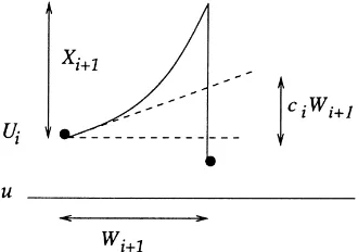
Fig. 3. Linear approximation to the surplus process.
where we have usedλz/(c+δz)≤λ/δfor allz≥0 and (8). Therefore,P˜[τ =n+1|Un]≥p0>0 and the bound p0is independent ofUn≥0, which implies thatτ is stochastically dominated by a geometric random variable with
parameterp0. Since a geometric random variable is finite a.s., thenP˜[τ <∞]=1 under the new measure.
By definition ofλnandRn, it follows that(λE[eRnY]/λn)≡1. Proceeding as before, we now obtain:
P{τ =n+1} = ˜E
( n
Y
i=1
e−(λ−λi)Wi+1eRiYi+11
{τ=n+1} )
= ˜E
(
exp
( n
X
i=0 λi−λ
ci
[ciWi+1−Yi+1]
)
1{τ=n+1} )
≤ ˜E
(
exp
(
λ0−λ c
n
X
i=0
(ciWi+1−Yi+1)
)
1{τ=n+1} )
.
From (1)ci = ddtU (Ti)is the initial slope of the surplus process at timeTi, so thatciWi+1≤Xi+1for eachi≤τ
(see Fig. 3.). ThusPni=0(ciWi+1−Yi+1)≤ Un+1−u, which yields the a.s. bound of 1 for the random variable
inside the expectation above. Adding overnwe obtain the estimator:
ψ(u, λ)= ˜E
"
exp
(τ−1 X
i=0
(λi−λ)
Wi+1− Yi+1
ci
)#
. (9)
3. Derivatives ofφ (X(t ), tφ (X(t ), tφ (X(t ), t≥≥≥000)))
Several approaches have been proposed to estimate gradients using only one simulated trajectory of the system, as in Brémaud and Vázquez-Abad (1992), Fu and Hu (1992), Glasserman (1991), Glynn, (1987), Pflug (1990), Reiman and Weiss (1989), among others. The main difficulty is that the functionalψ(u, λ)depends on the path in a non-linear way and the processN (t )is a.s. discontinuous inλ. The phantom RPA (rare perturbation analysis) estimators are applicable to this problem. We shall present our derivation of the method based on the results of Brémaud and Vázquez-Abad (1992), Baccelli and Brémaud (1993), and Vázquez-Abad (2000).
3.1. RPA for the storage process
Consider the general caseδ ≥0. Let{Xλ(t ), t >0}now denote the storage process (2) when claims arrive at
rateλ, so that the ruin probability is given by (3). It follows (see Fig. 1) thatDn =φ[Xλ(t );t ∈ [Tn−1, Tn)] for
Let{ηi}be a sequence of i.i.d. Bernoulli variables with parameterp =1λ/λ, also independent of{(Ti, Yi)}.
Think of 1λ > 0 as a “small” perturbation of the claim rate. Consider a process where the ith claim is dis-regarded iff ηi = 0 (it “disappears” and it is called a “phantom claim”). Since the thinned arrival process
thus obtained is a Poisson process with parameter λ−1λ, then the corresponding phantom process has the same distribution as {Xλ−1λ(t )}. We call nominal process the one for which all claims are honored:
ηi ≡1.
Under some regularity assumptions onG, the stationary derivative is the (uniform) limit of the finite horizon one and the following interchange in the limits is justified by Theorem 4 of Vázquez-Abad and Kushner (1992), as explained in the arguments that follow.
∂
for somes >0, this Markov chain satisfies a Doeblin condition (see Revuz, 1975) implying Harris recurrence. The phantom process for1λ >0 is stochastically dominated by the Harris recurrent process atλ, implying tightness of the set of invariant measures for(λ−1λ, λ]. Using the Radon–Nikodym derivative of the transition probabilities of the phantom process with respect to the nominal, the derivatives of the first step transition probabilities are uniformly bounded on compact sets. Under these conditions, Theorem 4 in Vázquez-Abad and Kushner (1992) can be applied to establish (10). Furthermore, convergence is at a geometric rate along the subsequenceTn → ∞,
yielding exponential convergence int.
Lett <∞be fixed and consider the finite difference in (10), calledψ1(λ, t ). Conditioning on the events that there aremphantomsηi =0 among theN (t )claims,
whereEmis the conditional expectation with respect to{ηi}givenN (t )andmphantoms among theN (t )claims.
For any fixedt, as1λ→0 the contribution of the sum above overm≥2 vanishes a.s., sinceN (t )has a bounded variance for finiteλ, andφ[Xλ(s);s ≤ t]≤ t a.s. (see the details in Vázquez-Abad (2000)). Therefore the only
term that survives in the limit ism=1, for which:
∂
is the corresponding quantity in the system where claimjis the only one disappearing. To obtain (11), use the fact that givenN (t )and one phantom, any one of theN (t )can be the chosen one with probabilityN (t )−1, so that
E{N (t )E1φ[X(s), s ≤t]} =EPN (t )j=1φ[Xj(s), s≤t]
andXj denotes the phantom system where exactly and
only claimjhas disappeared.
IfE[τ4]<∞then the rate of convergence of the derivative estimator isO(1/√t ). Indeed,Dn(0)−Dn(j )=0 ifn
andjindex claims belonging to different regenerative cycles (see Section 3.1 for details on the phantom processes). Furthermore, by definition Dn(0)−Dn(j ) ≤ 2τk(j ) if k(j ) indexes the regenerative cycle where j belongs.
276 F.J. V´azquez-Abad / Insurance: Mathematics and Economics 26 (2000) 269–288 We develop the general formulas for the phantom RPA derivative estimation, although our conditions simplify when we chooseλ0=λ+cR. Recall the definition of the cycle length (4) and identify now:
φ[U (t );t ≤τ]=K0τeµ(cTτ−Sτ),
whereK0 = (λ/Kλ0), so thatψ(u, λ) = ˜Eλ0{φ[U (t );t ≤ τ]}, whereK0 = (λ/Kλ0). We shall assume that E[eµY]<∞.Exwill now denote the expectation of the process when accidents occur at a ratex, but all claims
have thefixeddistribution with densityg(y)˜ =eµyg(y),µ=(λ0−λ)/c. We assume that there existsǫ >0 such that:
sup
where the remainder termR(1λ)is:
R(1λ)=eµ(cTτ−Sτ)
Consider the Poisson processN (t )with rateλ0and define{ηi}as a sequence of i.i.d. Bernoulli variables with
parameter 1−λ0/1λ, as well as the corresponding phantom systems. Then the surplus process obtained when
phantom claims are not considered has exactly the desired distribution for evaluatingψ(u, λ−1λ). Nowτ (η)
becomes a function of the sequenceη= {ηi, i≤τ (0)}, and we denote byτ (0)the nominal stopping time where no
claims are disregarded. Notice that there is now stochastic domination of the nominal system by the phantoms, in the sense thatτ (0)≤τ (η)(ruin will happen no later in the nominal system than in a phantom where some claims have not been paid). Conditioning on the sets ofmphantoms as before, the finite difference satisfies:
ψ1λ(λ0)=Eλ0
It can be shown (see Brémaud and Vázquez-Abad, 1992; Vázquez-Abad, 1999) that
Form≥1 the contribution of the remainder term will vanish in passing to the limit, which is shown as follows. Notice that by definition ofτ,eµ(cTτ−Sτ)<1 a.s. Next, letf (λ)=λ/(C+λ)whereC=λ
0−λis kept constant.
Using Taylor expansion with remainder, for any integerm:
∃ξ ∈(λ−1λ, λ) s.t. f (λ)m=f (λ−1λ)m+1λmf(λ+ξ )m−1 ∂
∂λf (λ+ξ )
which in turn implies thatkR(1λ)/1λk ≤(1/λ−1/λ0)τ (η)(K0)τ (η)a.s. Form=1, this term is multiplied by
the probability of 1 phantom, itself bounded a.s. byτ (0)1λ/λ0, while form≥2 it is multiplied by a term bounded
a.s. byτ (0)21λ2. Our assertion now follows from assumption (12) and dominated convergence.
Using thatτ (0) ≤τ (η)a.s, andφ ≤1 a.s., from assumption (12) and dominated convergence, it follows that only the termsm=0,1 are left in passing to the limit1λ→0.
For the termm=0 (no phantoms occur) the nominal and phantom paths coincide. Therefore, only the contribution of the remainder term survives in the limit form=0. Recall thatφ <1 a.s. and we have(λ−1λ)/K(λ0−1λ) < λ/Kλ0. As before,C =(λ0−λ)is a fixed scalar. Then, using(1−1λ/λ0)τ (0)→1 a.s., and dominated convergence,
it follows from our assumption that
− lim
Finally, the termm=1 is treated in an analogous way as for the storage process, yielding:
∂
The virtual RPA formula of Baccelli and Brémaud (1993) follows from a similar analysis as the phantom one, only this time we considerλ+1λ, where1λ >0, so that:
where the remainder termR(1λ)is now:
R(1λ)=eµ(cTτ˜−Sτ˜)
whereτ˜is the time of ruin for the process with Poisson arrivals at rateλ0+1λ. This arrival process has the same
distribution as a process where claims arrive from two independent sources: one which is Poisson at rateλ0and a
“rare” source with rate1λ. Claims coming from this source are called “virtual” claims. Naturally, for the process with only the Poisson arrivals, ruin cannot occurbeforeit happens when we add the virtual claims. Given thenominal process{(Wi, Yi), i =1, . . . , τ}withWi ∼exp(λ0), the probability of havingmvirtual claims within [0, Tτ] is
e−1λTτ(1λT
278 F.J. V´azquez-Abad / Insurance: Mathematics and Economics 26 (2000) 269–288
whereEmnow denotes the expectation conditioned on havingmvirtual claims. The arrival epochs of the virtual
customers, given onlymof them occur within [0, Tτ] follow the joint distribution ofmindependent uniform random
variables in [0, Tτ] (Taylor and Karlin, 1994). The limit as1λ→0 is:
where nowE1is the expectation under a uniformly distributed arrival epoch of the virtual customer.
Remark 2. The virtual RPA method can of course be applied to the storage process as well, which we state without further detail. Nonetheless, for the storage process the phantom systems are dominated, that is, they are below the nominal process w.p.1 (see Section 3), while the virtual processes would dominate the nominal system, meaning that some of the virtual claims may cause two or more cycles to merge. Domination by the nominal system is a desired property, first because it allows us to bound the variance of the estimators in precise terms, but also for practical purposes when executing the programming codes. For this reason, we have chosen to present the virtual RPA for the surplus process, where with probability one, ruin cannot occur sooner in the virtual systems than in the nominal process.
3.2.3. Interest model
We will illustrate the virtual RPA for the interest rate model (9), assuming that the claim distribution is exponential. Other distributions can be treated similarly, as long as they satisfy the assumptions. Define
hn=exp
virtual RPA method by considering a process with arrival rateλ+1λ, for1λ >0. The change of measure (8) of Section 2.2.2 prescribes usingλn=cnβ. Instead, we useλn+1for the change of measure, to be able to write
measure will also ensureP1λ-a.s. finite ruin epochs.
At each claim epochTn1λ, givenUn1λ, the next interarrival time for the1λ-process has an exponential distribution with rateλn+1λ, so it has the same distribution as the random variable min(Wn+1, Vn+1), whereWn+1∼exp(λn)
andVn+1∼exp(1λ)is independent ofWn+1and all previous random variables. Furthermore, it follows from the
lack of memory of exponential random variables that the residual life ofV1givenV1> Tn1λis also exponential with
parameter1λ. Therefore the distribution of the1λ-process is the same as the following process. LetV1∼exp(1λ)
and callτ1 =min{n:Wn > V1−Tn1λ−1}, where the distribution ofWn+1 ∼exp(λn)depends on the state of the 1λ-processUn1λ. SetWn1λ =Wn, n < τ1, Wτ11λ =V1, V2∼exp(1)independent of all the other variables, and
τ2=min{n > τ1:Wn> V2−Tn1λ−1}, Wn1λ =Wn, τ1< n < τ2, etc. Notice that the epochsτi are stopping times,
Use now the fact thatV1, V2, . . . are interarrival times of a Poisson process with rate1λ. These are the
vir-tual claims. Given the nominal process {(Yi, Wi), i = 1, . . . , τ}, the probability of having mvirtual claims is
e−1λTτ(1λT
τ)m/m! For the termm =0, with probability e−1λTτ → 1, the nominal and virtual paths coincide
and the finite difference is only due to the remainder term:
R(1λ)
For the termm=1, the contribution of the remainder term vanishes, since the probability of one claim is of order O(1λ). Similarly, the contribution vanishes as1λ→0 form≥2, sincehτhas finite expectation. The virtual RPA
formula becomes now:
where as in (9)E˜refers to the expectation under the measure determined by (8), andE1is the conditional expectation
w.r.t. a uniformly distributed arrival timeT∗∼U[0, Tτ] of the virtual claim,h˜τ˜is the corresponding statistics.
4. The phantom and virtual estimators
We shall now describe how we can estimate the derivatives via the “phantom” estimators in (11),(13),(14) and (16). Our method is based on an efficient way to calculate these quantities in parallel, thus using common random numbers. The phantom estimators for the interest model of the surplus process is presented in detail first.
4.1. Phantom storage processes
We have chosen to illustrate the more difficult case whenδ >0. The analysis for the linear caseδ=0 follows in exactly the same manner and we leave it to the reader. Fig. 1 shows one regenerative cycle of a typical path of the process. Let{Xn(0)}denote the nominal process (2) sampled only at the event times when accidents occur. Then
this process is Markovian, and from (2) it follows the recursions:
Xn+1(0)=
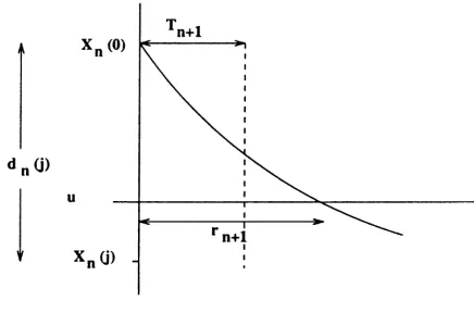
Furthermore, as in Michaud (1993), ifrn+1denotes the residual time needed for the ODE in (2) to attain levelu
if there were no further claims and the initial condition was set atXn(0), then:
rn+1=
280 F.J. V´azquez-Abad / Insurance: Mathematics and Economics 26 (2000) 269–288
Fig. 4. Pathwise construction of phantom systemj=3.
Define thedifference processas:
dn(j )=Xn(0)−Xn(j ).
Clearly,Xn(j )=Xn(0)for alln < j. At the epochTj, we setXj(j )=Xj(0)−Yj. The difference process then
satisfiesdn(j ) =0, j > n, dj(j ) =Yj. It is easy to see thatdn(j )are decreasing a.s., and thatXn(j )≤ Xn(0),
as shown in Fig. 4. Therefore ifXn(0)=0, necessarilyXn(j )=0 and by the next claim, the two processes will
coincide. This means thatdn(j ) >0 only fornwithin the regenerative cycle wherejbelongs. The difference process
can then be calculated recursively (see Fig. 4) by taking into consideration only one cycle at a time:
dn+1j =
e−δWn+1d
n(j ), if Xn(0)−δc(eδWn+1−1) > dn(j ),
e−δWn+1 X
n(0)−cδ(eδWn+1−1), otherwise
since in the first situation the phantom storage process is positive in the whole interval, and otherwiseXn+1(j )= Yn+1.
Remark 3. Notice that the evolution of the nominal process as well that of each of the phantom systems is inde-pendent of the value of u.
Our goal is to calculate Zn(j ) = Dn −Dn(j ). We use the difference process to do this. Notice first that
ifXn(0)≤ uthen all nominal and phantom systems will remain belowu for the whole interval [Tn, Tn+1)a.s,
andZn+1(j )=0. Otherwise,Xn(0) > uand we distinguish two cases. Ifdn(j ) > Xn(0)−uthen, as shown in
Fig. 5,Dn+1(j )=0 and therefore in this caseZn+1(j )=min(Wn+1, rn+1).
The case wheredn(j ) < Xn(0)−uis illustrated in Fig. 6. IfWn+1is smaller than the residual time until thejth
phantom system reaches levelu, calledrn+1(j ), thenDn+1(j ) =Dn+1=Wn+1, otherwiseDn+1(j )=rn+1(j )
andDn+1(0)=min(Wn+1, rn+1). In both this situations, we haveZn+1(j )=(min(Wn+1, rn+1)−rn+1(j ))+.
Fig. 6. Phantom systems: case 2.
Finally, a straightforward calculation gives
rn+1(j )=rn+1+
1
δln
1− dn(j )
Xn(0)+c/δ
.
4.2. Phantom surplus processes
The phantom systems resulting from disregarding any particular claim are quite easy to construct. We need to evaluate one cycle of the nominal surplus process under the new reference measure, containing a random number
τ of claims. For each claim, we consider the corresponding phantom system, as illustrated in Fig. 7.
As soon as the claim amountYj, j≤τ is generated, the differencedj(j )=Yjbetween the nominal surplus and
the phantom surplus is calculated. Since both processes evolve following the linear dynamics, thendn(j )=Yjfor
alln≤τ. Having omitted the payment of one claim, clearly the phantom surplus is always larger than the nominal, which means thatτ (j )≥τ (0). Using our previous notation, the amount by which the nominal process falls below zero at the moment of ruin isS(0)−cT(0). IfS(0)−cT(0) > Yj, thenτ (0)will also be the epoch of ruin for thejth
phantom system and we say that it “dies”. At epochτ (0)we calculate the contribution(τ (0)/λ)K0τ (0)eµ[cT (0)−S(0)].
If there are any phantom systems still “alive”, we keep generatingWnandYnand keep only one quantitycTn−Snas
would correspond to the nominal system. Again, at any moment, ifcTn−Sn > Yjfor each living phantom indexed
byj ≤τ (0), then this system dies and we can thus add its contribution(K0τ (j )/λ0)eµ[cT (j )−S(j )]to (13).
282 F.J. V´azquez-Abad / Insurance: Mathematics and Economics 26 (2000) 269–288
4.3. Virtual surplus processes
In order to implement (14) a direct approach prescribes generating one cycle of the surplus process under the measure with rateλ0and Esscher transform of the claims as in Section 2.2.1, keeping in memory all the values {(Wi, Yi)}of the trajectory. OnceTτis known, generateT∗∼U[0, Tτ] as the arrival epoch of the virtual customer,
and its claim amountY∗with densityKeµyg(y). To calculate the estimator (14) it is now necessary to backtrack
and re-calculate the virtual trajectory once the virtual customer is added into place, to computeτ , T˜ τ˜andSτ˜.
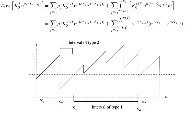
But backtracking a simulation is not numerically efficient. Instead, we propose to generate in advance the virtual claim sizeY∗. There are two types of intervals: ifU (t ) > Y∗ then the virtual claim will not cause the ruin if
t < T∗ ≤ Tτ (n), whereτ (n)is the index of the first claim afterwards such thatUτ (n) < Y∗, as illustrated in Fig.
8 for intervals of type 1. Rather,τ˜ =τ (n)in this case. On the other hand, intervals of type 2 are those where the surplus processU (t )is belowY∗. IfT∗belongs to one of these intervals, then ruin is immediate,Tτ˜ =T∗, Sτ˜ =Sn
andτ˜ =n+1 wherenis the index of the claim just prior toT∗.
Define the break pointsκi as follows: setκ0=0, τ (1)=0. Supposeu < Y∗, setκ1=min(W1, (Y∗−u)/c).
WhileUn< Y∗, n≥1 (which means thatκn=Wn), and setτ (n)=τ (n−1)+1,Z(n)=(Tτ (n)−1, Sτ (n)−1−Y∗).
Next,κn+1=Tn+min(Wn+1, (Y∗−Un/c). Onceκn< Wn, we enter an interval of type 1. Setτ (n)=1+min{n≥
τ (n−1):Un < Y∗}, so thatκ(n)=Tτ (n)−1. Until the (τ (n)−1)st claim the process will remain aboveY∗and
virtual claims happening within this interval of time will all have the effect of causing the ruin atκ(n). SetZ(n)= (Tτ (n), Sτ (n)−Y∗). Then repeat calculating intervals of type 2 with the associatedZn. CallIi the set of indicesn
such that(κn, κn+1] is an interval of typei=1,2.
When the simulation is over we knowTτ. A na¨ıve approach would be to generate a uniform random variable on
[0, Tτ] and look for the indexnsuch thatκ(n) < T∗≤κ(n+1). If this interval is of type 1, setTτ =Z1(n), Sτ˜ =
Z2(n)+Y∗,τ˜=τ (n), if it is of type 2, then setTτ˜=T∗, Sτ˜=Z2(n)+Y∗,τ˜ =τ (n).
A conditioning argument can further reduce the variance of the estimation (Ross, 1997). Callρj =κj −κj−1.
GivenY∗and the nominal trajectory{(Wi, Yi), i =1, . . . , τ}, ifT∗belongs to an interval of type 1, the desired
statistics is independent of the actual value ofT∗, while if the interval is of type 2, the conditional expectation can be evaluated analytically:
TτE1
h
K0τ˜eµ(cTτ˜−Sτ˜)
i
=X
j∈I1
ρjK0τ (j )eµ(cZ1(j )−Z2(j ))+
X
j∈I2
Z κj
κj−1
h
K0τ (j )eµ(ct−SZ2(j ))dt
i
=X
j∈I1
ρjK0τ (j )eµ(cZ1(j )−Z2(j ))+
X
j∈I2
K0τ (j ) µc e
−µZ2(j )(eµcκj −eµcκj−1).
Unfortunately, for the interest model we cannot perform the integration to improve the efficiency of the method when using (16). Naturally, we can still condition the expectation according to the subinterval [Tn, Tn+1)where the
virtual arrival may occur.
IfT∗ > Tn1λ, then the two processes coincide up to thenth claim. On the other hand, sinceT∗ ∼U[0, Tτ],
P[Tn< T∗≤Tn+1]=Wn+1/Tτ, which yields:
TτE1[hτ˜]=
τ
X
j=1
Wj+1hjE(j )
τ (j )Y−1
i=j
e(λi(j )−λ)
Wi+1(j )−
Yi+1(j ) ci(j )
,
wherehj is defined by (15) NowE(j )is the expectation conditioned on arrival of the virtual customer atT∗ ∼
U[Tj−1, Tj], which naturally changes the evolution of the remainder of the process. In the simulations, we generate
a uniform variableWj(j )in(0, Wj] at each stage, and associate the claimYj(j ) = Yj as in the nominal. From
there on, we use common random numbers to generateWn+1andWn+1(j )as well asYn+1andYn+1(j ), which will
depend on the (distinct) state valuesUnandUn(j ). Under this construction, the virtual systems are dominated by
the nominal trajectory.
5. Simulation results
5.1. Functional estimation
The storage process and its various phantoms are independent of the initial endowmentu, as explained in Section 3.2. Therefore, a single run can be used to simultaneously estimate in parallelψ (·, λ), Ψ (·, λ)for a set of values of
u. To illustrate the gain in computational effort, forλ=1.0, estimating 10 values ofudoing 10 separate simulations took 36.75 s of CPU time, while estimating the same 10 values in parallel took 12.49 s. These experiments were performed in a Sparc Station 10. In addition to saving computer time and memory, we were able to estimate the ruin probability and its derivative as functions ofuusing common random variables, which smoothes out the variability. We illustrate functional estimation with the non-linear dynamics with interest rateδ =0.05 using the storage process with the RPA method. As shown in Gerber (1979), the ruin probability now satisfies Segerdahl’s formula:
ψ(u, λ)= Γ
λ δ, β
c δ +u
Γ λδ, βcδ+λδβcδ λ/δ e−βc/δ
,
284 F.J. V´azquez-Abad / Insurance: Mathematics and Economics 26 (2000) 269–288
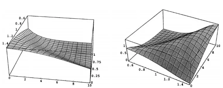
Fig. 10. Estimated functionsψ(u, λ)˜ andΨ (u, λ)˜ .
whereΓ (a, b)=Rb∞xa−1e−xdxis the incomplete gamma function. We do not have an explicit expression for the
derivativeΨ (u, λ).
Mathematicawas used to plot the ruin probablilityψ(u, λ)for a region in the(u, λ)plane. As for the derivative, direct differentiation caused numerical instabilities (aside from taking several minutes to compute). We had to use a sequence of finite differences, making the differences smaller yet avoiding numerical problems, until we were satisfied with our approximations, shown in Fig. 9. Therefore, our “theoretical values” for the derivatives are actually numerical approximations. It should be noted that solving this way for the derivative usingMathematicatook longer than running our simulations. The estimated surfaces are shown in Fig. 10.
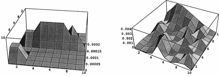
Finally, to illustrate a better measure of the over all efficiency of our estimators, we present in Fig. 11 the estimated mean square error of both the ruin probability and of its derivative.
5.2. Confidence intervals
For the surplus process with importance sampling a sequence ofNi.i.d. samples was simulated. For each sample we simulated one trajectory of the surplus process under the reference measure until the timeτ (0)of ruin, but we kept the simulation going until all the phantom systems also ruined. Since the estimators of bothψandΨ are then a sequence of i.i.d. variablesYi, we used the sample variance to estimate the standard deviation as well as our level
αconfidence intervals:
ˆ
For the storage process, we use the regenerative method Bratley et al. (1987) in order to estimate the (asymptotic) variance and the confidence intervals. Let Ci, Yi denote, respectively, the cycle length and cumulative statistics
P
nDnfor estimatingψ(orPnZnfor the derivativeΨ) over theith regenerative cycle. We usedNregenerative
cycles for the estimator. Define the statistics:
ˆ
By the renewal theorem,Vi =Yi −ψ Ciare i.i.d. mean zero random variables. Since they have bounded variance,
they satisfy the central limit theorem,
√
In the next sections we present the numerical comparison of the proposed methods for estimating the ruin probabilityψ(u, λ)and its derivativeΨ (u, λ). A common measure of comparison is theefficiencyof the estimators. If we callYNan estimator obtained withNreplications of the simulation, we define its efficiency as being the inverse
of the product of its variance and mean CPU time:
E= 1
CN(Var(YN)+β(YN))
, (19)
whereβNis the bias of the estimator andCNthe mean CPU time associated. The Importance Sampling estimators
are unbiased and the Storage Process estimators are strongly consistent. We therefore estimate the asymptotic efficiency assuming “large” sample sizes and estimating the efficiency by:
ˆ
E= 1
ˆ
CNV ar(Yd N)
,
where the estimated variance is the same as the one used to build the confidence intervals.
In all our experiments we used functional estimation for the storage process, therefore we had to adjust the formula for the efficiency (19) in this case, multiplying by the number of different values ofureported (in this case, 4). This accounts for the fact that the CPU time of a single simulation yields the 4 estimations at once, while the importance sampling performs one simulation for each value ofuand the CPU time is dependent onu.
5.3. The linear dynamics
We first report the simulation results for the linear dynamics, whenδ=0. We usedY1∼exp(1/β)for the claim
286 F.J. V´azquez-Abad / Insurance: Mathematics and Economics 26 (2000) 269–288
ψ(u, λ)= 1 θexp
−
θ
1+θ
u β
, Ψ (u, λ)≡ ∂
∂λψ(u, λ)=
1
λψ(u, λ)
u β(1+θ )+
1+θ θ
,
whereθ=c/λβ−1>0 (otherwiseψ(u, λ)=1).
For the surplus process under importance sampling we choseλ0 =λ+Rc, so thatK0 =1 and the likelihood
ratioφ[U (t );t ≤τ]≤1 a.s. which bounds the variance of the estimator uniformly. We now proceed to justify this choice. For the exponential claim model, the new distribution is exponential with parameterα−µ, forα =1/β
provided that:
1
β >
(λ0−λ)
c ⇒λ0< c β +λ
so thatEˆλ0[Y]=1/(α−µ). We must chooseλ0so that ruin is certain under the new measure, that is, we want λ0> c/Eˆλ0[Y], which yields:
λ0> c
β −(λ0−λ) ⇒λ0>
1 2
c β +λ
.
Finally, for this modelλ+Rc=c/β, which always lies in the desired interval, since we assumedλ < c/β. The following table gives the simulation lengths.
Number of cycles for estimatingψ(u)
Importance sampling 100,000
Storage Process 300,000
Number of cycles for estimatingΨ (u)
Phantom IS 50,000
Virtual IS 70,000
Phantom SP 300,000
In Table 1 we give the results forψˆX,ψˆUandΨˆX,ΨˆUfor the linear case. The estimators are identified by “X” or
“U”, whether they correspond to the storage process (SP) or to the surplus process under importance sampling (IS). Subindices “UP”, “UV” and “XP” refer to the phantom or virtual RPA method. We report the confidence interval (CI) forα=0.05.
The length of the cycles (and thus the computational effort) depends onuwhen using importance sampling, which naturally tends to work better for larger values ofu, when estimating probabilities of a “rarer” event than for
u=0. For the storage process the situation is very different. On one hand, one single simulation yields all values ofu, but naturally the variance of the estimator becomes larger (in general) for larger values ofu. While it seems at first glance that importance sampling has smaller variance for all the estimators than the indirect estimation method, once the computing time is taken into account, it seems that the second estimator may be more efficient in some situations.
In addition, simulations using importance sampling strongly depend on the model and the particular claim distribution. It is not evident that for other distributions ofYi, including empirical distributions, we can choose an
optimal value ofλand a “good” change of measure forYi. In Vázquez-Abad and LeQuoc (2000) we experiment
Table 1
Linear dynamics:δ=0
u=0 u=2 u=4 u=6
Ruin probabilityψ(u)
ψ(u) 0.66667 0.34228 0.17573 0.09022
ˆ
ψU(u) 0.6669±0.0014 0.3422±0.0007 0.1759±0.0003 0.0904±0.0002
Eff 359,550 1,369,808 5,170,465 19,640,353
ˆ
ψX(u) 0.6670±0.0018 0.3420±0.0027 0.1751±0.0025 0.0898±0.0020
Eff 1,200,782 532,937 609,213 977,867
Derivative of ruin probabilityΨ (u)
Ψ (u) 0.66667 0.79864 0.64435 0.45112
ˆ
ΨU P(u) 0.6713±0.0153 0.7997±0.0133 0.6394±0.0089 0.4515±0.0057
Eff 16,359 7,225 12,045 23,478
ˆ
ΨU V(u) 0.6698±0.0120 0.8000±0.0106 0.6465±0.0070 0.4549±0.0043
Eff 26,286 17,096 25,512 49,858
ˆ
ΨXP(u) 0.6669±0.0019 0.7968±0.0086 0.6389±0.0121 0.4437±0.0129
Eff 817,048 40,895 20,895 18,408
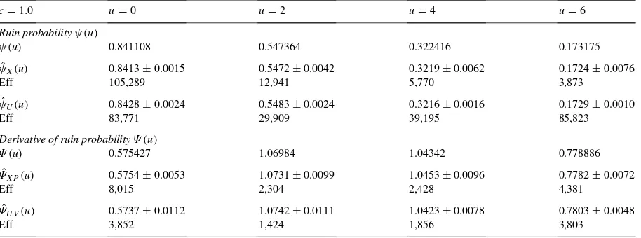
5.4. The dynamics with interest
We turn now to the caseδ >0 andβ =E[Y]=1.0. As before, we use exponentially distributed claim amounts in order to compare with the theoretical values. We considered firstλ = 1.0 and the two scenariosc =1.0 and
c=1.5 withδ=0.05, usingN =200,000 cycles for SP andN =50,000 cycles for IS. 95% confidence intervals are given in Table 2 forc=1.0 and in Table 3 forc=1.5.
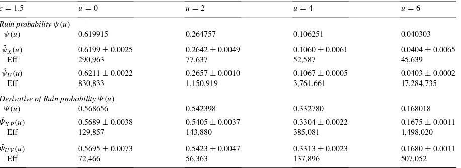
These results seem to indicate that, while estimation of ruin probabilities may be more efficient using importance sampling, especially for larger values ofu, this is not the case when estimating the derivatives. Recall that the virtual method was constructed for the particular example of exponential claims. When other distributions are used, it is not clear how the method should be adapted. In particular, evaluation of the implicit equation forRi
is required at each step of the simulation, a task that may be numerically very heavy. On the other hand, the
Table 2
Exponential dynamics:δ=0.05
c=1.0 u=0 u=2 u=4 u=6
Ruin probabilityψ(u)
ψ(u) 0.841108 0.547364 0.322416 0.173175
ˆ
ψX(u) 0.8413±0.0015 0.5472±0.0042 0.3219±0.0062 0.1724±0.0076
Eff 105,289 12,941 5,770 3,873
ˆ
ψU(u) 0.8428±0.0024 0.5483±0.0024 0.3216±0.0016 0.1729±0.0010
Eff 83,771 29,909 39,195 85,823
Derivative of ruin probabilityΨ (u)
Ψ (u) 0.575427 1.06984 1.04342 0.778886
ˆ
ΨXP(u) 0.5754±0.0053 1.0731±0.0099 1.0453±0.0096 0.7782±0.0072
Eff 8,015 2,304 2,428 4,381
ˆ
ΨU V(u) 0.5737±0.0112 1.0742±0.0111 1.0423±0.0078 0.7803±0.0048
288 F.J. V´azquez-Abad / Insurance: Mathematics and Economics 26 (2000) 269–288
Table 3
Exponential dynamics:δ=0.05
c=1.5 u=0 u=2 u=4 u=6
Ruin probabilityψ(u)
ψ(u) 0.619915 0.264757 0.106251 0.040303
ˆ
ψX(u) 0.6199±0.0025 0.2642±0.0049 0.1060±0.0061 0.0404±0.0065
Eff 290,963 77,637 52,587 45,639
ˆ
ψU(u) 0.6211±0.0022 0.2657±0.0010 0.1067±0.0005 0.0403±0.0002
Eff 830,833 1,150,919 3,761,661 17,284,735
Derivative of Ruin probabilityΨ (u)
Ψ (u) 0.568656 0.542398 0.332780 0.168018
ˆ
ΨXP(u) 0.5689±0.0038 0.5405±0.0037 0.3304±0.0022 0.1675±0.0011
Eff 129,857 143,880 385,081 1,498,020
ˆ
ΨU V(u) 0.5695±0.0073 0.5423±0.0047 0.3313±0.0023 0.1680±0.0011
Eff 72,466 56,363 137,896 507,052
phantom RPA method with the storage process is very robust and does not require any special model dependent code.
Acknowledgements
Supported in part by NSERC-Canada grant # WFA0139015 and FCAR-Québec grant # 93-ER-1654. Computer simulations were prepared by Phong Le Quoc.
References
Asmussen, S., 1985. Conjugate processes and the simulation of ruin problems. Stochastic Processes and their Application 20, 213–229. Asmussen, S., Nielsen, H., 1995. Ruin porbabilities via local adjustment coefficients. Journals of Applied Probability 32, 736–755.
Baccelli, F., Brémaud, P., 1993. Virtual customers in sensitivity and light trafic analysis via campbell’s formula for point processes. Advances in Applied Probability 25, 221–234.
Bratley, P., Fox, B., Schrage, L., 1987. A Guide to Simulation, 2nd ed. Springer, New York.
Brémaud, P., Vázquez-Abad, F., 1992. On the pathwise computation of derivatives with respect to the rate of a point process: the phantom RPA method. Queueing Systems 10, 249–270.
Dufresne, E., Gerber, H., 1989. Three methods to calculate the probability of ruin. ASTIN Bulletin 19, 79–90
Fu, M.C., Hu, J., 1992. Extensions and generalizations of smoothed perturbation analysis in a generalized semi-markov process framework. Institute of Electrical and Electronics Engineers. Transactions on Automatic Control 37 (10), 1483–1500.
Gerber, H., 1979. An introduction to risk theory. Monograph 8, University of Pennsylvania, Philadelphia. Huebner Foundation. Glasserman, P., 1991. Gradient Estimation via Perturbation Analysis. Kluwer Academic, Boston.
Glynn, P., 1987. Likelihood ratio gradient estimation: an overview. Proceedings of the 1987 Winter Simulation Conference 336–375. Kleinrock, L., 1976. Queueing Systems. Wiley, New York.
Michaud, F., 1993. Estimating the probability of ruin of variable premiums by simulation. ASTIN Bulletin 26 (1), 93–105. Pflug, G.C., 1990. On line optimization of zimulated markov processes. Mathematics of Operations Research 15, 381–395. Reiman, M., Weiss, A., 1989. Sensitivity analysis for simulations via likelihood ratios. Operations Research 37, 830–844. Revuz, D., 1975. Markov Chains. North-Holland, Amsterdam.
Ross, S., 1997. Simulation, 2nd ed. Academic Press, Boston.
Siegmund, D., 1976. Importance sampling in the monte carlo study of sequential tests. Annals of Statistics 4, 673–684. Taylor, H., Karlin, S., 1994. Introduction to Stochastic Processes. Revised edition. Academic Press, New York. Vázquez-Abad, F., 2000. Convergence rates of the phantom RPA estimators for stationary sensitivities, to be submitted.
Vázquez-Abad, F., Kushner, H., 1992. Estimation of the derivative of a stationary measure with respect to a control parameter. Journal of Applied Probabilities 29, 343–352.