DETERMINING OF AN EXTREMAL DOMAIN FOR THE
FUNCTIONS FROM THE S-CLASS
by
Miodrag Iovanov
Abstract. Let S be the class of analytic functions of the form f(z) = z + a2 z2 +…, f(0)= 0, f′(0)=1 defined on the unit disk z <1. Petru T. Mocanu [2] raised the question of the determination max Re f(z) when Rez f′(z)=0, z = r, r>0 given. For solving the problem we shall use the variational method of Schiffer-Goluzin [1].
Key words: olomorf functions, variational method, extremal functions.
1. Let S the class of functions f(z) = z + a2 z2 +…, f(0)= 0, f′(0)=1 holomorf and univalent in the unit disk z <1.
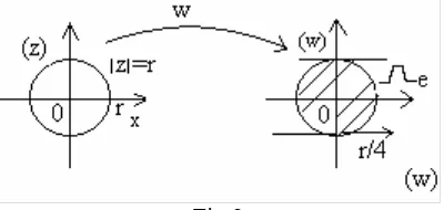
For the first time Petru T. Mocanu [2] brought into discussion the problem of determination the max Re f(z) when Rez f′(z)=0, z = r, r>0 existed.
Geometrically this is expressed like in the figure below:
2.Let z = r and let f
∈
S with Rez f′(z)=0, extremal function for exists the maximum max Re f(z), f∈
S. We consider a variation f∗(z) for the function f(z) given by Schiffer-Goluzin formula [1],(1) f*(z)= f(z)+
λ
V(z;ζ
;ψ
)+O(λ
2),ζ
<1,λ
>0ψ
real, where(2)
′
⋅
−
′
⋅
+
′
⋅
⋅
−
′
⋅
−
−
′
−
−
=
−
.
)
(
)
(
1
)
(
)
(
)
(
)
(
)
(
)
(
f(z)
)
(
)
(
)
(
e
)
;
V(z;
2 2
i 2 i
2 2
i
ζ
ζ
ζ
ζ
ζ
ζ
ζ
ζ
ζ
ζ
ζ
ζ
ζ
ζ
ψ
ζ
ψ ψ
ψ ψ
f
f
z
z
f
z
e
f
f
z
z
f
z
e
f
f
e
f
z
f
z
f
iIs known that for
λ
sufficiently small, the function f∗(z) is in the class S. We consider a variation z∗ for z:z∗ =z +
λ
h + O(λ
2), h=0 = ∗
∂ ∂
λ
λ
zwhere satisfy the conditions:
(3)
z
∗=
r
şi Re z∗f∗’(z∗)=0 Observing that :λ
2
2 2
+
=
∗
z
z
Re(z
h) +O(λ
2) = r2.Because z =r from relation (3) we obtain :
(4) Re (
z
h) = 0.Replacing z with z∗ in f∗(z) we have : z∗f∗’(z∗) = A +B
λ
+ O(λ
2) where :
+
+
=
=
)
;
;
(
'
)
(
''
)
(
'
)
(
'
ψ
ζ
z
zV
z
zhf
z
hf
B
(5) Re
{
h(f'(z)+zf"(z))+zV'(z;ζ
;ψ
)}
=0. Because f(z) is extremes we have:Re f∗(z*)
≤
Re f(z) where is equivalent with :Re
{
f(z)+λ
hf′(z)+L+λ
V(z;ζ
:ψ
)+L}
≤Re f(z) or(6) Re
{
hf′(z)+V(z;ζ
;ψ
)}
≤0.From (5) (
h
h
z
z
−
=
) and (6) we obtain:−
′
+
′′
+
′
(
)
(
))
(
;
;
)
(
f
z
z
f
z
z
V
z
ζ
ψ
h
h
(
f
(
z
)
z
z
′
+
z
⋅
f
′′
(
z
)
)+
z
⋅
V
′
(
z
;
ξ
;
ψ
)
=
0
from where:(7) h=
) ( )
( )
( )
(
) ; ; ( )
; ; (
2 2
2 /
z f z z f z z f z z f z
z V z z
V z z
′′ ⋅ + ′ ⋅ + ′′ − ′ −
′ +
⋅
ζ
ψ
⋅ζ
ψ
.
We will use the next denotations:
f= f(z), w=f(
ζ
) ,l
=
f
′
(
z
),
m =f
′′
(
z
)
,V = (z;ζ
;
ψ
), V′=VZ′(z;ζ
;ψ
). With previous denotations, the relations (6) and (7) can be writhed as follows:(8) Re
{
pzV ′+V}
≤0where p =
m z l z m z zl
l z zl
⋅ + ⋅ + −
−
⋅ −
2
2 (p real).
2 / 2 2 2 2 1 ⋅ ⋅ ⋅ ⋅ − ⋅ + ′ ⋅ ⋅ ⋅ − ⋅ − ′ ⋅ ⋅ − − ⋅ = − w w z l z e w w z zl e w w f e w f f e
V i i i i
ζ ξ ζ ζ ζ ζ ζ ψ ψ ψ ψ and + ⋅ ⋅ ⋅ −⋅ − ⋅ − − ′ ⋅ ⋅ ⋅ − −− ⋅ = ′ 2 / 2 2
2 ( )
) ( ) ( ) 2 ( w w z l m z z e w w l e w f w f fl e
V i i i
ζ ζ ζ ζ ζ ζ ψ ψ ψ + 2 / 2 2 . ) 1 ( ) 2 ( ) 1 ( ⋅ ⋅ ⋅ − − + ⋅ − − w w z z zl m z z e i ζ ζ ζ ζ ζ ψ .
Replacing in relation (8) the expression of V and V/ we obtain: (9) Re
[
e
iψ(
E
−
GF
)
]
≤
0
,
where:
[
]
[
]
[
]
′ = ⋅ − ⋅ ⋅ − ⋅ ⋅ + ⋅ ⋅ − − − − ⋅ ⋅ − + + + − ⋅ − − + = − + + − − = . ) 1 ( ) 2 ( ) 1 ( ) ( ) ( ) 1 ( ) ( ) 2 ( 2 2 2 2 2 2 2 2 w w F z z l z m z z pz z l m z z pz pzl z l z z zl f G w f pzlf f w pzl f f Eζ
ζ
ζ
ζ
ζ
ζ
ζ
ζ
ζ
ζ
ζ
ζ
(10)
[
]
= − + + − − ⋅ ⋅ ′ 2 2 2 ) ( ) 2 ( w f pzlf f w pzl f f w wζ
2 2 0)
1
(
)
(
ζ
ζ
ζ
⋅
−
−
∑
=z
z
t
k k k where[
]
[
]
⋅ − + − + = − − − − + + − + + − + + − − = + ⋅ + ⋅ + ⋅ + + + ⋅ − − + + + + ⋅ − + − + + = + − + − − − + + − = + + = .. ) ( ) ( ) 2 2 2 2 2 ( ) 2 1 ( ) 2 ( ) 2 1 ( 2 ) ( ) 2 ( 2 ) 2 ( ) 1 4 ( ) 2 ( ) 1 2 ( ) 1 4 ( ), 2 ( ) 1 ( 2 ) 1 ( 2 ) ( 2 4 4 2 4 2 2 2 2 2 2 2 2 3 4 2 2 2 4 4 2 2 2 4 2 2 3 2 2 2 2 2 1 2 0 z l lz z z z m p z f t l r m z r l z m mz z mr r pr r l z z zl r r z f t l z m r l z m r pz l mz zm r pz r r pzl r r l z r zl r r f t l z m pr m pz r plz l z l z r zf t f pzl f z tThe extremal function transforms the unit disk in the domain without external points. To justify this thing is sufficient to suppose that the transformed domain by an external function
w
=
f
(
ζ
)
has an external point w0 and to consider the function the variation: 0 2 *)
(
)
(
)
(
)
(
w
z
f
z
f
e
z
f
z
f
i−
+
=
λ
ψ ,λ
>0,ψ
real,f
*∈
S
3.Is known that the extrema function
w
=
f
(
ζ
)
transform the unit diskζ
< 1, in whole plane, cutted lengthwise of a finite number of analytically arc. Let q =e
iθ, the point of the circleζ
=1 where corresponding the extremity of this kind of section in whichw
/( )
q
=
0
andζ
=
q
is double root for the polynom∑
= 4 0 k k k
t
ζ
.Because
ζ
=
q
is double root for this polynom , we can write :∑
=40
k k k
From the relation about the coefficients tk ,
k
=
0
,
4
results that we can take.
,
2
,
1 2 2 40
0
t
a
kq
a
q
t
a
=
=
−
=
⋅
The differential equation (10) can be write:
(11)
[
(
)
]
(
)
( )
(
(
)
( )
1
)
.
2
1
2
2 2
2 4 2 0
2
2 2 2
ζ
ζ
ζ
ζ
ζ
ζ
z
z
t
q
kq
t
q
w
f
pzlf
f
w
pzl
f
f
w
w
−
−
+
−
−
=
−
+
+
−
−
⋅
′
4.After radical extraction in (11) we obtain:
(
)
[
]
)
1
)(
(
2
)
1
(
)
(
2
2 0 2 4 2ζ
ζ
ζ
ζ
ζ
ζ
z
z
t
q
kq
t
q
dw
w
f
w
pzlf
f
w
pzl
f
f
−
−
+
−
−
=
−
+
+
−
−
.
From double integration:
(12)
∫
[
(
)
]
=
−
+
+
−
−
w
dw
w
f
w
pzlf
f
w
pzl
f
f
0
2
)
(
2
∫
−
−
−
−
+
ζ
ζ
ζ
ζ
ζ
ζ
ζ
0
2 4 2 0
)
1
)(
(
2
)
1
(
z
z
t
q
kq
t
q
.
For calculation the integral from left side of (12) we denote:
=
1
I
∫
[
(
)
]
−
+ + −
−
dw w
f w
pzlf f
w pzl f
f
) (
2 2
. We observe that :
∫
+
−
−
−
=
dw
w
f
w
a
w
pzl
f
f
I
)
(
)
2
(
2
1 where we denoted .
2
2 2
a pzl f
pzlf f
= −
− +
For the calculation of I1 we make the substitution :
w
=
u
2−
a
2,
dw
=
2
udu
.
Weobtain
∫
=
+
−
−
−
−
−
=
b
a
f
b
u
a
u
du
u
pzl
f
f
I
2 2 2 2 22
1
,
)
)(
(
2
)
2
(
.2 2 2 2 2 2 2 2 2 2 2 2
1
2
1
2
)
)(
(
2
b
u
a
b
b
a
u
a
b
a
b
u
a
u
u
−
⋅
−
−
−
⋅
−
=
−
−
−
.So:
+
−
−
−
+
−
−
⋅
−
−
=
b
u
b
u
a
b
b
a
u
a
u
a
b
a
pzl
f
f
I
(
2
)
ln
ln
2 2 2
2
1
or
(13)
−
+
⋅
+
−
⋅
−
−
−
−
=
b a
b
u
b
u
a
u
a
u
a
b
pzl
f
f
I
1(
2 22
)
ln
where :
2
a w
u= + . For calculation the integral from right side of (12) we denote:
∫
−
−
−
−
+
=
ζ
ζ
ζ
ζ
ζ
ζ
ζ
d
z
z
t
q
kq
t
q
I
)
1
)(
(
2
)
1
(
0 2 4 22 .
We have:
q
2t
4ζ
2−
2
kq
ζ
+
t
0=
q
2t
4⋅
(
ζ
−
ζ
1)(
ζ
−
ζ
2)
where
.
4 4 0 2
2 ,
1
q
t
t
t
k
k
±
−
=
ζ
If we denotation k− k2 −t0t4 =δ
observe thatq
t
41
δ
ζ
=
and 0 .2 q
t
δ
ζ
=with this denotations, 2 ( )( 0 ).
4 4
2 0
4 2
q t q t t
q t kq t
q
δ
ζ
δ
ζ
ζ
+ = − −− For the
calculate the integral I2 make the substitution :
(14) ( )( ) ( )
4 0
4
q t v q t q t
δ
ζ
δ
ζ
δ
ζ
− − = − .(15)
1
2 2 2−
−
⋅
=
v
v
α
σ
ζ
withq
t
4δ
σ
=
and 2 024δ
α
=t t .By an elementary calculation from (15) obtained successively:
(16)
−
−
=
−
−
−
−
=
−
−
−
=
−
−
−
=
−
−
⋅
−
=
−
−
−
=
−
−
⋅
−
=
−
−
−
=
.
1
)
1
(
)
)(
(
1
1
cu
1
)
1
(
1
,
1
1
1
)
1
(
1
,
cu
1
)
(
,
)
1
(
)
1
(
2
2 2 0 4 2 2 2 2 2 2 2 2 2 2 2 2 2 2 2 2 2 2v
v
q
t
q
t
ş
i
q
q
v
v
q
q
z
z
cu
v
v
z
z
z
z
v
v
z
z
dv
v
v
d
α
σ
δ
ζ
δ
ζ
σ
σα
δ
δ
σ
ζ
σ
σα
γ
γ
σ
ζ
σ
σα
β
β
σ
ζ
α
σ
ζ
By using previous relations we obtain:
(17)
∫
− − − − − − − − − = dv v v v v v v z z t q q I ) )( )( )( 1 ( ) ( ) 1 )( ( ) 1 )( 1 ( 2 2 2 2 2 2 2 2 2 2 2 4 2 2 2
γ
β
α
δ
σ
σ
σ
α
σ
. Let:)
)(
)(
)(
1
(
)
(
)
(
2 2 2 2 2 2 2 2 2 2γ
β
α
δ
−
−
−
−
−
=
v
v
v
v
v
v
v
F
;we are looking for a decomposition
(18)
γ
γ
β
β
α
α
+
+
+
−
+
+
+
−
+
+
−
+
+
+
−
=
v
A
v
A
v
A
v
A
v
A
v
A
v
A
v
A
v
F
1 2 3 4 5 6 7 81
1
)
(
.(19)
⋅ = − −
− −
= − =
= − −
− −
= − =
= − −
− −
= − =
= − −
− −
= =
4 2 2 2 2 2
2 2
8 7
3 2 2 2 2 2
2 2
6 5
2 2 2 2 2 2
2 2
4 3
1 2 2
2 2
1
) )(
)( 1 ( 2
) (
) )(
)( 1 ( 2
) (
) )(
)( 1 ( 2
) (
) 1 )( 1 )( 1 ( 2
1
τ
β
γ
α
γ
γ
γ
γ
δ
τ
γ
β
α
β
β
β
β
δ
τ
γ
α
β
α
α
α
α
δ
τ
γ
β
α
δ
A A
A A
A A
A A
We denote,
) 1 )( (
) 1 )( 1 (
2 2 2 4
σ
σ
σ
α
σ
µ
z z
t q
q
− −
⋅ − −
= ; from (18) and (19) we obtain
for I2 the expression:
(20)
+
−
+
+
−
+
+
−
+
+
−
=
γ
γ
τ
β
β
τ
α
α
τ
τ
µ
v
v
v
v
v
v
v
v
I
ln
ln
ln
1
1
ln
2 3 41
2 .
From the relation (14) observe that:
(21) ( ) ,
4 0
q t
q t
v
δ
ζ
δ
ζ
ζ
− −
=
v
(
0
)
=
±
α
and from
w
=
u
2−
a
2 we obtain:(22) ,
2 2 )
( ) (
2
pzl f
pzlf f
w u
+ + −
=
ζ
ζ
u
(
0
)
=
±
a
.(12/) ζ 0 2 0
1 I
I w=
For
ζ
=
0
from (13), (20) and (12/) obtained the constant (which is obtained from that two members of relations (13) and (20) corresponding toa
u
a
u
+
−
fromα
α
+
−
v
v
(from left)): 2 2 2
) 2 ( ) 1
ln( − +µτ
− −
− b a
pzl f f a
, obtained in left member of equality (12/). Thus, (12/) can be writhed:
( )
− = + − + − − − + − + ⋅ + − − − − + − − − 2 2 2 ) 2 ( 2 2 2 2 2 2 1 ln ln ) 2 ( ) ( ) ( ) ( ) ( ln ) 2 ( µτ ζ ζ ζ ζ a b pzl f f a b b a b a a b pzl f f b u b u a u a u a b pzl f f . 1 1 ln ) ( ) ( ln ) ( ) ( ln ) ( ) ( ln 1 ) ( 1 ) ( ln 4 3 1 4 3 2 1 +− + − ⋅ + − − − + − + + − + + − + + − = τ τ τ τ τ τ τ γ α γ α β αα β α α µ γ ζ γ ζ β ζ β ζ α ζ α ζ ζ ζ µ v v v v v v v vWith calculus the previsious equality can be writhed:
(23) + − ⋅ +− − + ⋅ + − ⋅ + − ⋅ +− = = − + ⋅ − + ⋅ + − − − − . ) ( ) ( ) ( ) ( ) ( ) ( 1 ) ( 1 ) ( ) ( ) ( ) ( ) ( 4 3 2 1 2 2 ) 2 ( µ τ τ τ τ
γ
α
γ
α
γ
ζ
ζ
γ
β
α
β
α
β
ζ
β
ζ
ζ
α
ζ
α
ζ
ζ
ζ
ζ
ζ
ζ
v v v v v v v v b a b a b u b u u a ua b a
pzl f f b a
extremal function
w
=
w
(
ζ
)
, where realized maxRe f(z).S
f∈
II. We suppose that
Im(
zl
+
z
2m
)
=
0
.
In this case the expression of p, have to zl−zl =0. How zl+zl =0 implies zl=0. If l=0(z =r >0) then l =0. From (6) results thatw
(
ζ
)
have to verify the condition:(24)
Re
0
/ 2
≤
−
−
w
w
f
w
f
f
e
iζ
ψ .
How
ψ
is arbitrary, real, results thatw
(
ζ
)
verify next differential equation:(25)
w
f
f
w
w
−
=
2/
ζ
.or
ζ
ζ
d
w
f
w
dw
f
=
−
. From double integration:(26)
∫
=
∫
−
w
d
w
f
w
dw
f
0 0
ζ
ζ
ζ
.With denotation f −w =t, obtained
w
=
f
−
t
2,
dw
=
−
2
tdt
.
The relation (26) becomes (without limits of integration):∫
=∫
⋅ −
−
ζ
ζ
d t t f
dt t f
) (
) 2 (
2 or
ln
,
)
(
2
2
2
ζ
∫
=
−
f
dt
t
f
from where
ζ
ln
ln
=
+
−
f
t
f
t
(27)
ζ
ζ 00
ln
ln
=
+
−
−
−
wf
w
f
f
w
f
.
After the calculus we obtained successively:
ζ
=
−
+
−
ζ
+
+
−
−
−
ζ
−
ζ
=
+
−
−
−
−
+
−
−
−
= ζ
= ζ
ln
w
)
f
w
f
(
ln
f
w
f
f
w
f
ln
and
,
ln
ln
f
w
f
f
w
f
ln
f
w
f
f
w
f
ln
0 2
0 0
from where:
ζ
ln
4
ln
=
⋅
−
+
−
−
f
w
f
f
w
f
f
and
(28)
f
w
f
f
w
f
f
4
ζ
=
−
+
−
−
.
From (28) we obtained:
(29) 2
2
)
)
(
4
(
)
(
16
)
(
z
z
f
z
zf
z
w
+
=
.How f(z) is considerate the extremal from (29) obtained after some calculus that
4
)
(
z
z
Fig 2
and the condition
Re
zw
/(
z
)
=
0
impliesx
=
0
(
z
=
x
+
iy
)
.Then
z
=
max
Re
w
(
z
)
=
0
, so forz
e=
0
and ∀z > ze,any parallel to Ox intersected f(z =r) in one point.We exclude this ordinary case, it showing that the problem is true.
From I and II, result that the extremal function which is corresponding to the extremal region
Ω
e from fig 1, has the implicitly form in equation (23).5.Still remain to show how to determine the
θ
. For this we make in (11);
z
→
ζ
and after simplifications and by multiplication of equality fromz
3l
we obtained:(
t
kqz
q
t
z
)
z
l
z
q
p
l
l
r
r
3(
2−
1
)
⋅
=
(
1
−
)
2 0−
2
+
2⋅
4⋅
2⋅
3⋅
or :
(30) ( 1) ( ) ( 2 2)
4 2 2 0
2 2 2
3 r ll p z qr t zl kqlr q t lz r
r − ⋅ = − − + ⋅ .
Because p is real,
r
3(
r
2−
1
)
l
l
p
,
is real from the relation (30) we obtain a system with two equation and determinateθ
and k :(31)
(
)
[
]
(
)
[
]
=
+
−
−
+
−
−
=
−
0
)
2
(
Im
)
2
(
Re
)
1
(
2 4 2 2 0
2
2 4 2 2 0
2 2 2
3
zr
l
t
q
r
l
kq
l
z
t
r
q
z
zr
l
t
q
r
l
kq
l
z
t
r
q
z
p
[image:13.595.224.424.87.182.2]With
θ
and k determinated in this way the extremal function from equation (27) is well determine and with its assisting we find z maxRe f(z)w f
e = ∈ with the
geometrical property enounced: in domain
Ω
e=
{
z
z
>
z
e}
,
any parallel to the Ox axis intersect f(z =r)in one point (eventually in maximum one point).References
[1].G.M. Goluzin, Geometriceskaia teoria complecsnogo peremenogo, Moscva-Leningrad, 1952.
[2].Petru T. Mocanu, O problemă extremală în clasa funcţiilor univalente, Universitatea Babeş Bolyai-Cluj Napoca, Facultatea de Matematică, 1998.
Author: